Transient structural analysis (also known as dynamic analysis) is a method used to determine the dynamic response of a structure over time. Through the analysis of transient analysis, we can obtain the time-dependent results such as displacement, strain, stress, and reaction force of the structure under the arbitrary combination of steady-state loads, transient loads, and harmonic loads. The biggest advantage of transient analysis over the static analysis is that it considers inertia and damping effects.
Common analysis methods for transient problems are:
- Time-domain transient analysis
- Eigenvalue extraction (natural frequency and modal)
- Steady-state response (harmonic response analysis in the frequency domain)
- Spectrum response analysis (peak response calculation of shock)
- Random response analysis (vibration caused by random excitation)
Because the time-domain transient method is the most intuitive, it can solve a variety of linear and nonlinear problems, and has been applied often in the industry. This article only introduces the time-domain transient method. Other methods will be introduced in the future.
Governing equation
The fundamental equation of motion for transient dynamics is:
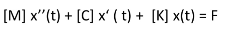
Where [M] is the mass matrix. [C] is the damping matrix. [K] is the stiffness matrix. {u_tt} is the nodal acceleration. {u_t} is the nodal speed. {u} is the nodal displacement. {F} is the load. It can be seen that the transient structural governing equation is an equation containing second-order time derivatives. There are many methods for solving the second-order time derivative. The most widely used in the structural finite element is the Newmark implicit time integration method. WELSIM’s default time solver for structural analysis is also the Newmark method.
Common solving methods
There are three common finite element methods for transient dynamics: full method, reduced method, and modal superposition method.
The full method uses complete system matrices to calculate the dynamic response. It is the most powerful and supports solving various nonlinear characteristics such as plasticity, large deformation, large strain, etc. The advantage is that it is easy to use and you don’t have to concern about choosing the principal degree of freedom or vibration mode. The scheme allows various types of nonlinear characteristics. The full matrix is used, no mass matrix approximation is involved. Displacements and stresses over all-time history can be obtained in one single analysis. All types of boundary conditions are allowed. The main disadvantage of the complete method is that it is expensive, time-consuming, and the solved data is large.
The reduced method compresses the data size by using a principal degree of freedom and reduced matrices. As the displacements at the principal degrees of freedom are calculated, the solution is extended to the complete set of degrees of freedom. The advantage is that it is faster and less expensive than the full method. The disadvantage is that the initial solution only calculates the displacement of the principal degrees of freedom. Only nodal boundary conditions can be applied to the model. All loads must be added to the principal degrees of freedom. The size of the time step must be constant. The automatic time stepping is not supported. Nonlinearity is not supported (except node-to-node contact).
The modal superposition method calculates the structural response by multiplying the mode shapes (eigenvalues) obtained by the modal analysis and summing them. The advantages are: faster and less expensive than the reduced or full method. It allows the modal damping (damping ratio as a function of the vibration model). The disadvantage is that the size of the time step must be constant and the automatic time stepping is not supported. Nonlinearity is not supported (except node-to-node contact). Non-zero displacement boundary conditions cannot be applied.
Because of the superiority of the full method and its wide application in linear and nonlinear problems. This article only discusses the full method.
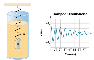
Damping
Considering the effect of damping is one of the advantages of transient analysis. Damping can be regarded as a kind of energy dissipation, which comes from many factors. In the finite element analysis, damping is often regarded as an overall effect and is applied using numerical algorithms.
There are three common damping settings in FEM: direct damping, Rayleigh damping, and composite damping. Direct damping can define the critical damping ratio related to each order mode, and its typical value range is between 1% and 10% of critical damping. Rayleigh damping assumes that the damping matrix is a linear combination of the mass and stiffness matrices. Although the assumption that damping is proportional to the mass and stiffness matrix has no sufficient physical basis, we know very little about the distribution of damping, and practice has proven that Rayleigh damping is effective in the finite element analysis thus is widely used. Composite damping can define a critical damping ratio according to each material so that the composite damping value corresponding to the overall structure is obtained. Composite damping is more effective when there are many different materials in the structure.
In most linear dynamic problems, accurately defining damping is important for results. However, the damping algorithm and parameters only approximate the energy absorption characteristics of the structure, not the physical mechanism that causes this effect in principle. Therefore, it is difficult to determine the damping data in the finite element analysis. Sometimes we can obtain these data from experiments, sometimes we have to refer the material manual or experience to determine the damping parameters.
Time solver
For transient structural problems, due to the introduced second-order time derivatives, we need a time solver. Generally, we divide time solver into two categories: explicit solvers and implicit solvers.
The explicit solver uses the results of the previous and current steps to calculate the next result. Explicit solver has unstable regions and requires a small time step. The advantage is that you do not need a nonlinear solver (Newton’s iterative solver) to solve nonlinearity, and you do not need to assemble a stiffness matrix. At the same time, the encoding and algorithm are relatively simple. It does not require additional memory to store the intermediate data. The stable step size of the explicit solver can be estimated, but due to the complexity of the actual calculation, the practical time step usually is smaller than the theoretical step size. Explicit algorithms require that the mass matrix must be diagonal. The advantage of solving speed shows only when the number of finite elements is small. Therefore, the reduced integration method is often used, which easily triggers the hourglass mode and affects the calculation accuracy of stress and strain. The representative algorithms of the display solver are the central difference, forward Euler, Runge-Kutta, linear acceleration method, etc.
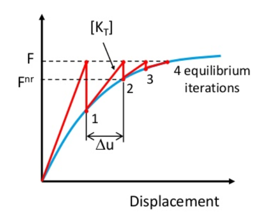
The implicit solver iterates the next step result with the current step result and the next unknown result, which must be obtained through iteration. The implicit solver requires the assembly of a stiffness matrix, and Newton iteration is required to solve nonlinearity. The commonly used methods are the Newmark method and Wilson-Theta method. The variant algorithms can be implemented by modifying the alpha, beta and theta parameters in the algorithm. For example, the calculation efficiency and accuracy of the HHT solver on some problems have been significantly improved. The biggest advantage of the implicit solver is that it has unconditional stability, that is, the time step can be arbitrarily large. However, we need to take a reasonable time step in the actual practice. At the same time, some solvers such as Newmark have second-order accuracy.
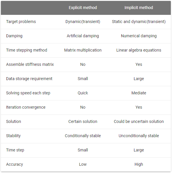
Comparison of explicit and implicit solvers as shown below
In order to ensure the full response of the structure and ensure the stability and convergence of the solution, it is important to choose the correct time step. Generally speaking, the smaller the time step, the more accurate the solution. However, a smaller time step leads to a large number of solving steps, and the physical computation time will increase significantly. Therefore, the size of the time step cannot be too small. Meanwhile, the time step cannot be too large, otherwise, the calculation will miss many high-order frequencies of the structure, leading to unrealistic solutions.
Automatic time stepping is an automatic algorithm that can optimize the computation in transient problems. The user only needs to set the initial step, maximum and minimum step sizes. During the solution process, the solver will automatically reduce the time step as required to calculate any rapid changes in the motion. In the process of slow change in motion, the solver can increase the time step, thereby improving the calculation speed.
Boundary and initial conditions
Unlike static analysis, it is due to the characteristics of transient and inertia. The transient analysis supports velocity and acceleration boundary conditions. These boundary conditions, especially acceleration, can be used to simulate the effects of excitation.
For initial conditions, the transient analysis generally supports the following three:
- Linear static results. It specifies the initial displacement of the structure under a certain load.
- A transient analysis result that determines the transient response of the structure at a certain moment. Solving can begin at any specified time step.
- The initial velocity and initial acceleration of all free nodes in the structure.
The initial velocity condition is a more common initial condition, and it is often applied to all nodes of a structure to mimic moving bodies.
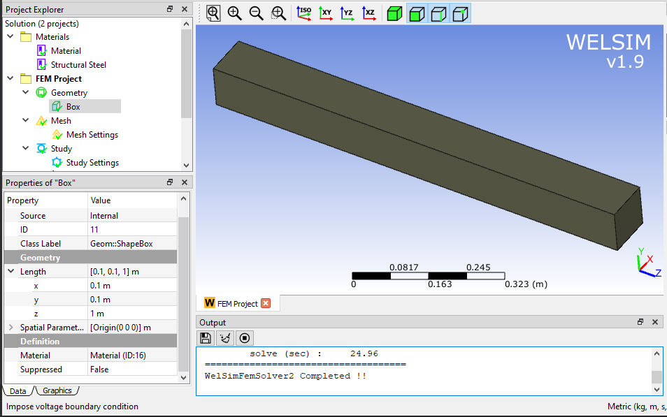
The above is the core knowledge in terms of structural transient analysis. Below we look at how to implement finite element analysis in software WELSIM.
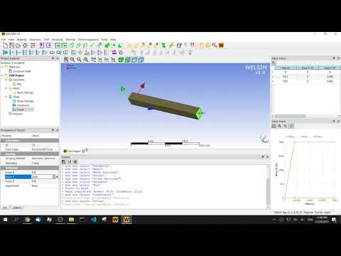
Structural transient analysis steps
1) Create or import a model
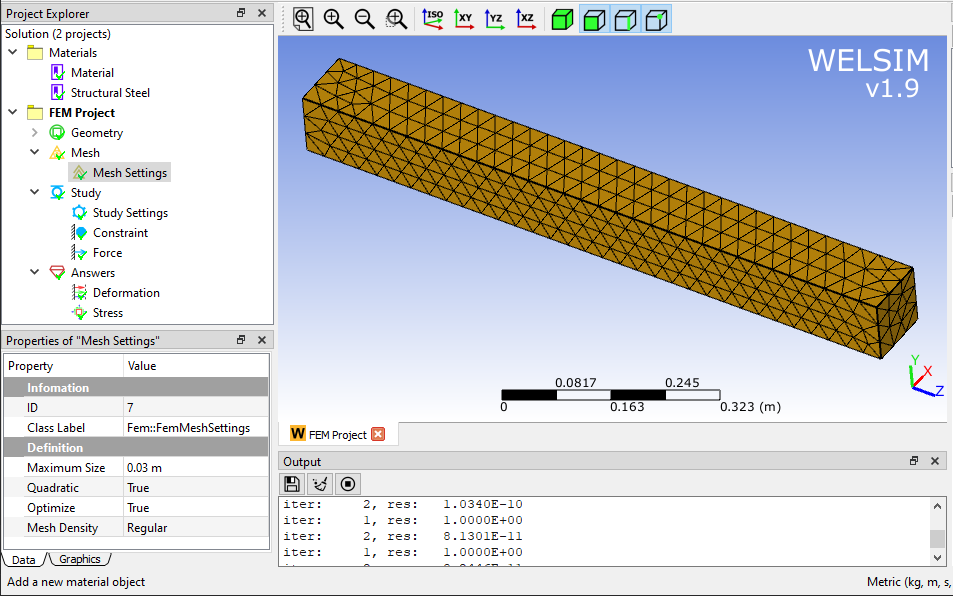
2) Meshing
3) Load step and time step settings
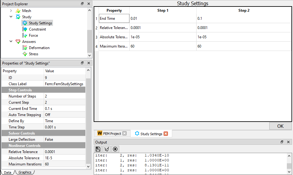
Number Of Steps: Load steps, which specify the number of load steps in this analysis. Current Step: The current load step. Current End Time: The end time of the current load step. Auto Time Stepping: Whether automatic time stepping is on. WELSIM currently only supports fixed step sizes for structural analysis, so this option is turned off by default. Define By: The way to define the load substep. It can be defined by time and the number of substeps. Time Step: The size of the time step. Available when Defined By is set to Time.
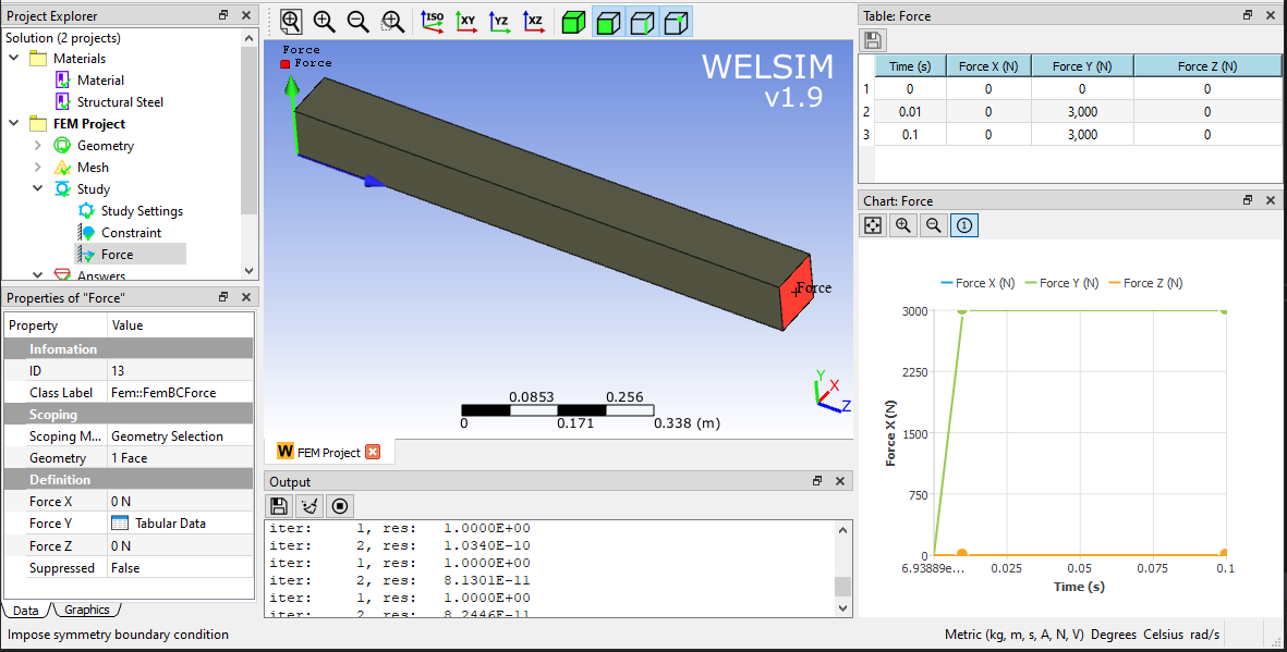
4) Set boundary conditions, initial conditions, contacts, etc.
5) Solve and verify results
The figure below shows the maximum and minimum deformations in the Y direction and von-Mises stresses over the entire time history.
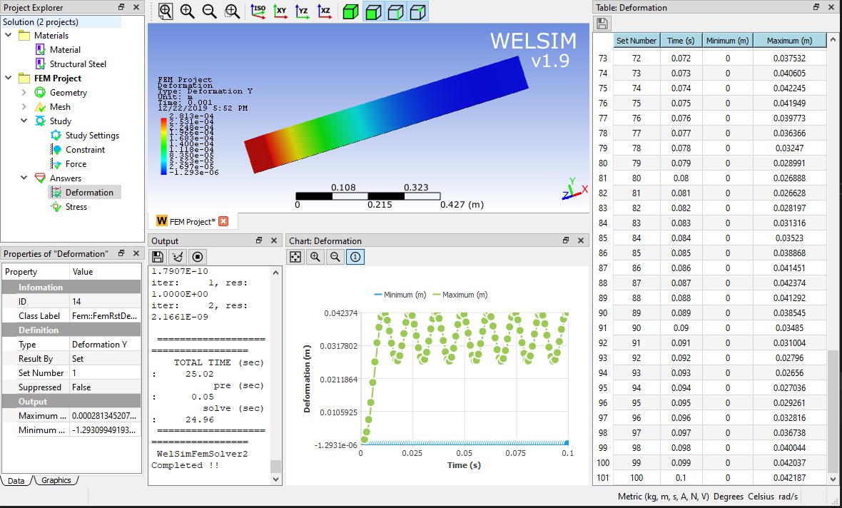
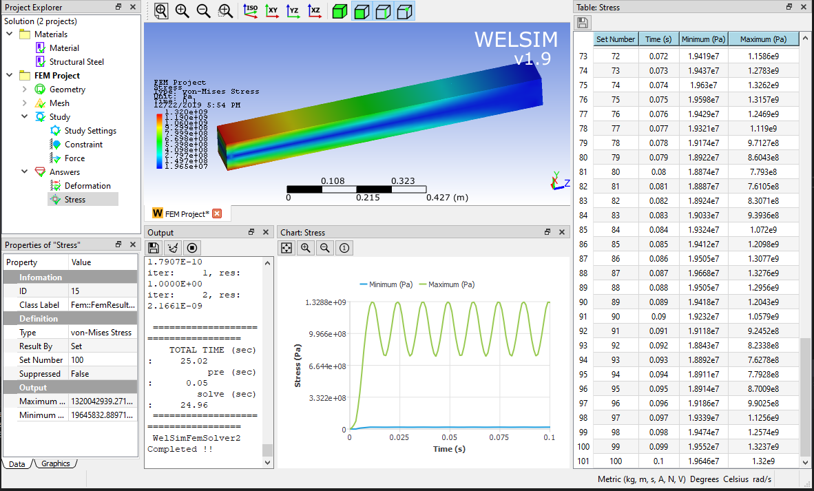
It can be seen that no damping occurs in this analysis because of no attenuation of the reciprocating vibration. The role and setting of damping will be introduced in the future.
Finally, the operation video is provided for your reference.