With the development of finite element analysis technology, engineers are no longer satisfied with the one single step static analysis. To better understand the structural dynamics of the system, we will use transient analysis methods. The transient finite element analysis can directly solve the dynamic response in the entire time history, but the calculation and output of the full deformation and stresses at each time step will inevitably lead to long calculation time and huge result files. Therefore, we often perform a static analysis of structures or systems at multiple load steps, also known as quasi-static analysis, to help us quickly understand the system and its response to external forces.
Multi-step quasi-static analysis
Although the quasi-static does not exist in practice, it is of great significance in engineering practice as a basic mechanical model. Many practical problems can be approximated as quasi-static problems and meet engineering accuracy requirements. The quasi-static analysis considers the change of boundary conditions in terms of time, and can obtain the system or structure response under different external conditions. Especially for nonlinear problems involving contact, collision, plasticity, creep, expansion, viscoelastic materials, multi-step quasi-static analysis can quickly obtain approximate results. For those dynamic problems in which the system inertia is negligible, the results of the quasi-static analysis can be directly used in engineering practice.
It is worth noting that quasi-static analysis ignores the effects of inertia, damping, and frequency. For systems or structures whose inertia cannot be ignored, the quasi-static analysis also provides a reliable numerical reference for our next-level transient analysis.
The steps
In multi-step finite element analysis, two important concepts about steps are often encountered:
Step: Generally refers to the load step. In the analysis, the entire loading process is divided into several sequential steps; for example, when analyzing elastoplastic problems, the first step is loading and the second step is unloading. The loading process can also be broken down into Multiple Steps, but usually, this can be achieved by multiple Substeps in the solution process.
Substep: If nonlinearity occurs at each load step, to solve it, a load step is decomposed into multiple substeps to ensure that each substep converges and finally achieves step convergence.
Schemes in multi-step quasi-static analysis
In the quasi-static analysis, each load step is calculated independently and has nothing to do with the previous and next load steps. Although it appears that subsequent load steps are calculated based on the previous steps, each step calculation is based on the initial configuration of the structure. You can solve it directly based on your constraints and loads in this step, without considering the first load step. The structural response only corresponds to your material, constraints and loads, regardless of the load steps before and after.
Common analysis steps
To better understand multi-step, let’s take a look at how to set up a multi-step analysis on the finite element software. This case uses a simple cantilever beam as an example. The external force varies with the steps or time. The basic steps are:
- Geometry Modeling
- Finite element meshing
- Set the number of load steps
- Set multi-step boundary conditions
- Solve, and evaluate results
It can be found that no matter whether it is a linear analysis or a nonlinear analysis, the processing of multi-step analysis is very similar to the single-step analysis. The only difference lies in the setting of the number of load steps and the setting of the boundary conditions for each step.
Examples
In the following example, we use finite element software WELSIM to implement the multi-step quasi-linear analysis.
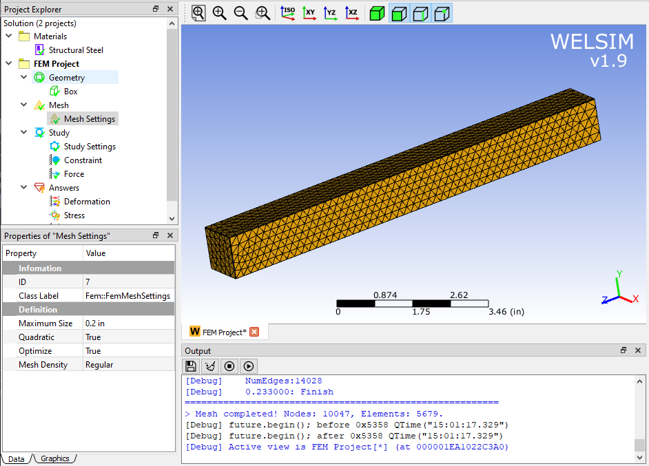
Add 3D box geometry and set the length, width, and height to 1’’x1’’x10’’.
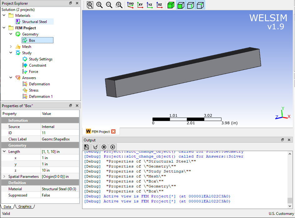
In the mesh settings, set the maximum element size to 0.2’’ and use the Quadratic setting to generate Tet10 elements.
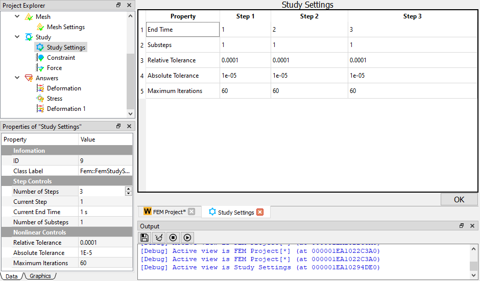
The major difference between the multi-load step and single-load step analysis is the difference in the number of load steps. In this example, we set three load steps. In the analysis settings, set the Number of Steps to 3. Double-click the Study Settings object. You can see that the corresponding settings under all load steps are displayed in the pop-up table, and the rest properties remain the default.
One end of the beam is fixed.
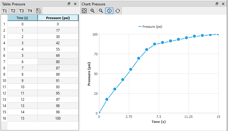
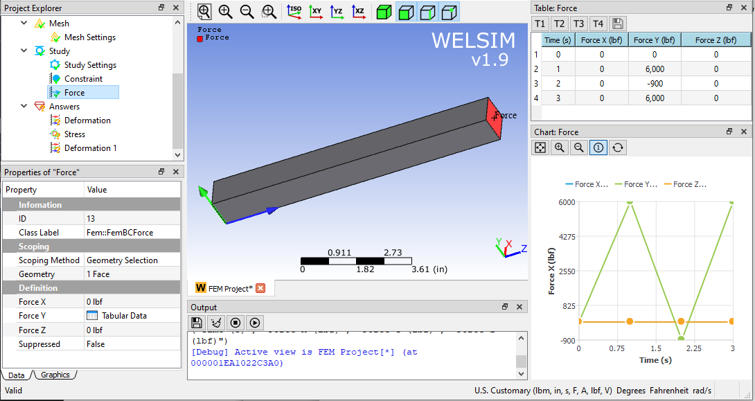
At the other end of the beam, because the force varies with time, the property window of the boundary condition is no longer sufficient for the input of values. You need to enter the corresponding values for the load steps and dimensions in the table window. Here a force of 6000, -900, 6000 lb is applied to each load step in the Y direction. Forces in other directions are zero.
After setting the boundary conditions, click Solve and get the results soon.
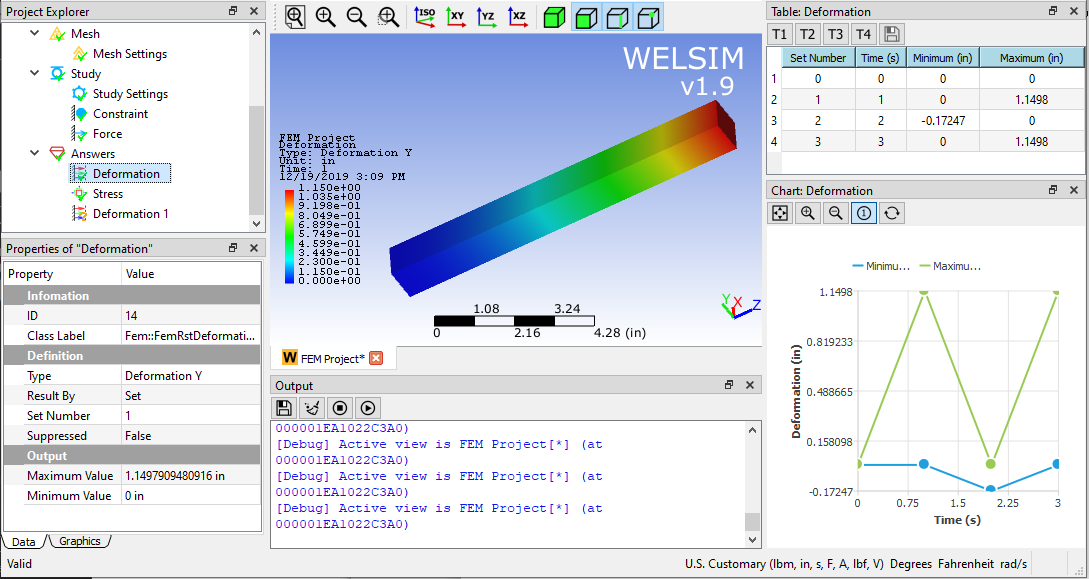
Deformation in the Y direction under the first load step.
Von-Mises stress results in the first load step.
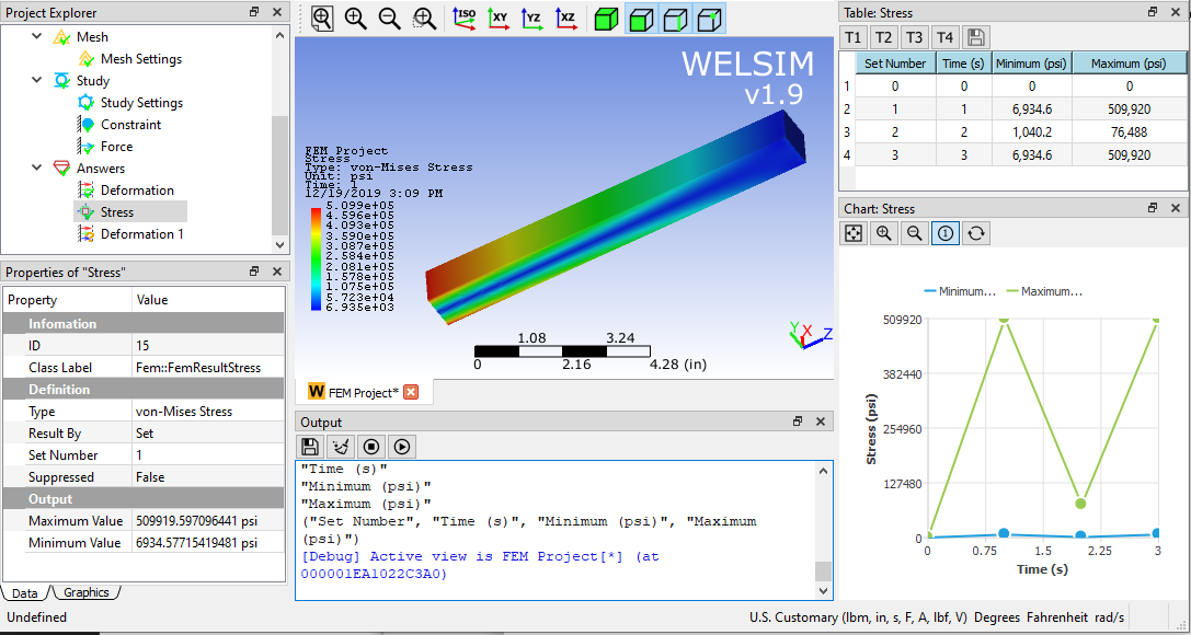
It can be seen that due to changes in boundary conditions, deformation and stress also fluctuate. The results of the first load step and the third load step are consistent, indicating that the effects of inertia and frequency are ignored in quasi-static. However, as a fast and convenient method of variable load analysis, the multi-step quasi-static method contributes a lot to engineering design, prediction, and analysis.
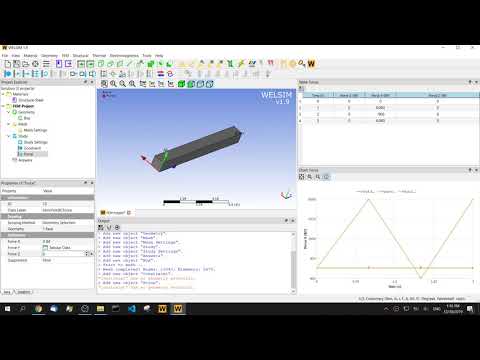
Finally, attach the operation video for your reference.