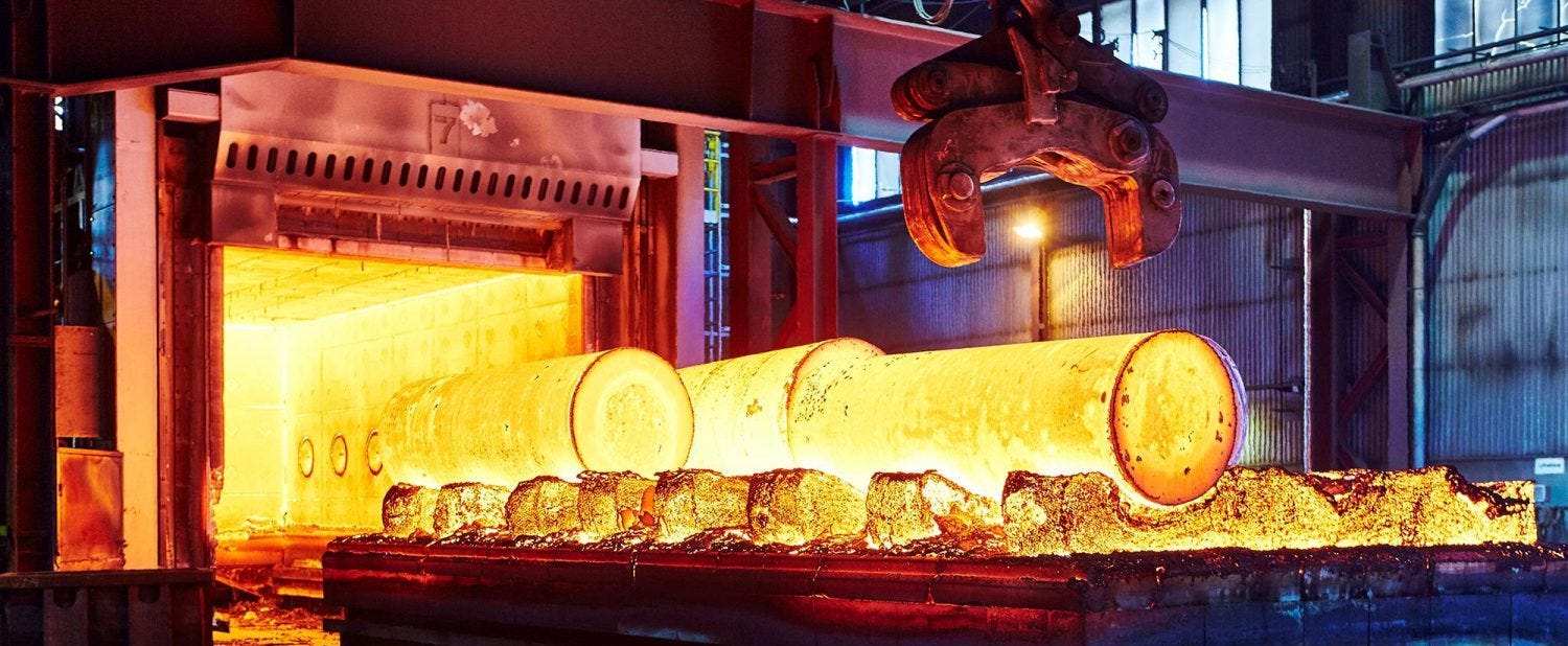
Thermal (also called heat transfer) analysis is one of the commonly encountered analyses in engineering. Thermal analysis is used to predict or verify the temperature distribution on structural parts at specific heat conditions. Once the thermal characteristics are determined from simulation, the thermal performance of the product can be optimized by changing the position of the heat source, improving the heat dissipation methods, or applying thermal insulation, etc.
With the development of computer-aided engineering (CAE), the finite element method has become one of the most important methods for heat transfer analysis. Like other types of analysis, there are a large number of nonlinear conditions in the heat transfer process. Although some processes can be simplified to linear problems. there are still many thermal nonlinearities that we need to consider during the analysis.
There are three common nonlinearity types in heat transfer analysis:
Temperature-dependent material properties
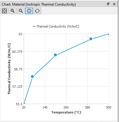
This is one of the most common nonlinearities in thermal problems, the material properties show nonlinearity in terms of temperature changes. The nonlinear thermal material properties could be thermal conductivity, specific heat, density, and enthalpy. In the steady-state analysis, only thermal conductivity parameter participates in the calculation, while transient problems also need to consider specific heat and mass density.
Temperature-dependent boundary conditions
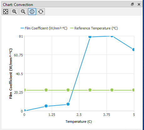
Another nonlinearity is caused by temperature-dependent boundary conditions. The Common boundary conditions in heat transfer analysis are temperature, heat flow, heat flux, convection, and radiation. Based on the actual physical conditions, each of those boundary conditions may exhibit nonlinearity in terms of temperature changes.
Radiation boundary condition
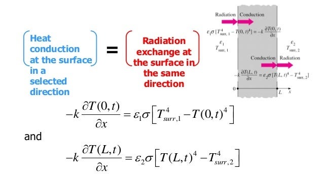
Radiation is a highly nonlinear boundary condition. For plane radiation, the heat transfer is proportional to the fourth-order of the temperature difference between the plane and the ambient. The physical mechanism of radiation is complicated. In engineering, we use Stephan constant, emissivity coefficient, and ambient temperature to depict the radiation process. Since the Stephan constant is a fixed parameter (5.67032e-8 W/m²/K⁴), the user only needs to define the emissivity coefficient and ambient temperature in WELSIM. In a future article, we will explain the thermal radiation conditions in detail.
Solve the nonlinearity
The nonlinearity mentioned above can exist in either the steady-state or transient thermal analysis. Thanks to the implicit algorithms used in the finite element method, nonlinear problems are mostly iteratively calculated by Newton’s solver. In Newton’s iteration method, the iterative substep is used to obtain the result of each Newton iteration increment, and the next iteration is advanced until the calculated residual is less than a certain small value, then the convergence is reached. Line search is a useful algorithm for solver enhancement. For conditions where the heat transfer rate changes significantly, the activated line search can speed up convergence and improve precision. Thus the line search is suitable for strongly nonlinear problems. In WELSIM, users do not need to make special settings for the nonlinearity, the system will automatically determine nonlinearity and apply the optimal algorithms to solve.
When the nonlinearity presents, the convergence of computation becomes important. For models with strong nonlinearity, the default solver settings may not converge, and some parameters need to be adjusted to guarantee the convergence of the solving. The solver parameters that can be adjusted are:
- Reduce the load step size
- Reduce the time step size in transient analysis
- Adjust convergence criteria and number of iterations
If the model still does not converge even if a lot of parameters have been adjusted, it may be due to the strong nonlinearity for such physical problems. Fortunately, most nonlinear heat transfer models in engineering can be convergent.
Finite element analysis procedures
This section describes how to set up and solve a nonlinear heat transfer problem in the finite element software. These settings and steps work not only to the WELSIM software but also to most commercial finite element software.
- Define the materials needed in the model. If the material has thermal nonlinearity that changes with temperature, you need to define the relevant data in the table window, and the graph window will display the corresponding curve.
- Set the physics and analysis type.
- Import the model and generate the finite element mesh.
- For transient analysis, set time steps, initial conditions.
- Apply the initial temperature and boundary conditions. WELSIM thermal analysis supports 5 boundary conditions: Temperature, Heat flow, Heat flux, Convection, Radiation, and Insulated. One body condition: Internal Heat Generation, and one initial condition: Initial Temperature.
- Solver control settings, including convergence criteria, iteration termination conditions, etc. Due to the complexity of non-linear settings, it is recommended that you use the default settings at the first solve. If the solution does not converge, then adjust the solver parameters.
- Set the result output controls.
- Solve and evaluate the results.
Example
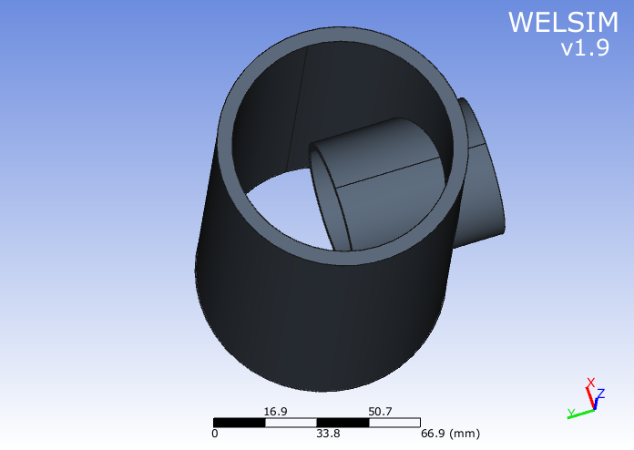
This example analyzes the tank duct under certain thermal conditions to understand the entire process in nonlinear thermal analysis. The temperature of the fluid in the tank is 450 degrees, which flows out through the small duct, and the temperature of the fluid in the small duct is 100 degrees. The structure is as follows:
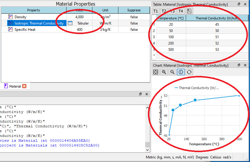
In the heat transfer analysis, the steady-state analysis needs to define the thermal conductivity of the material, and the transient analysis also needs to define the mass density and specific heat. If it is a thermal stress analysis, you also need to define the coefficient of thermal expansion. If some properties of the material are temperature-dependent, the user can enter corresponding values in the table window. The graph window displays the curve of the corresponding data. The Cell corresponding to material properties will display a special table icon to indicate that the property is represented by table data. As shown in the figure below:
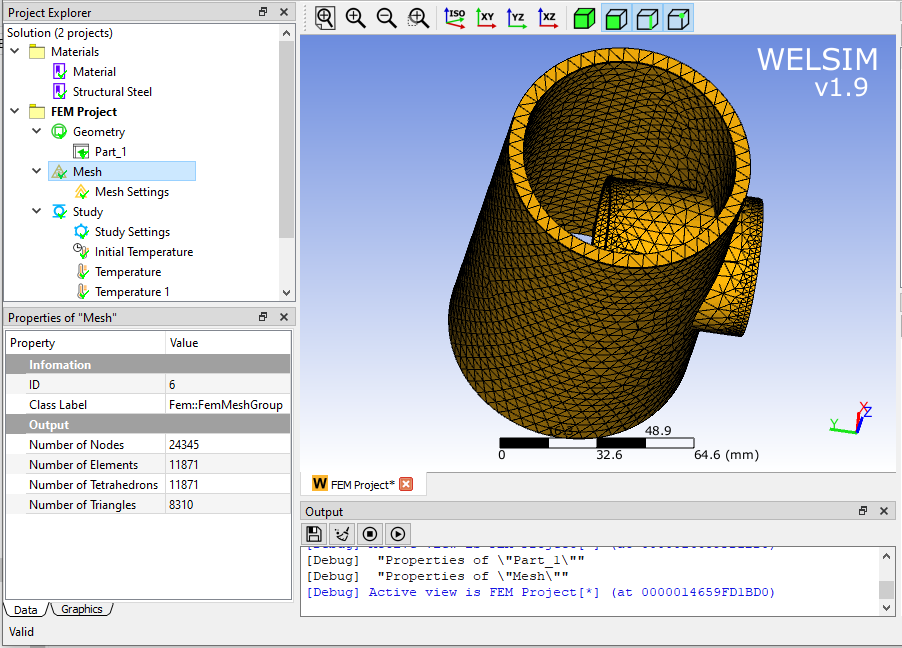
The imported model needs to be meshed. WELSIM supports automatic tetrahedral mesh. In this example, we use the high order Tet10 element. Click the mesh button. If the mesh is successfully generated, the mesh statistical data will be displayed in the properties view.
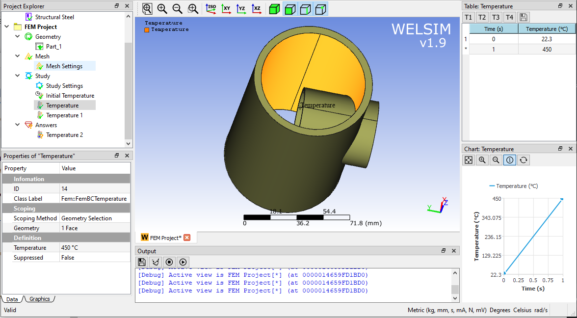
This example is to analyze the heat exchange on the structure surfaces, we need to specify the temperature boundary conditions on the surface. The boundary conditions defined here include the selected surface and magnitudes.
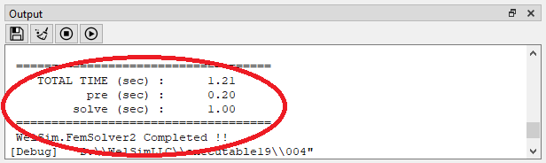
When the settings are completed, click Solve. If the setting is insufficient or the solving is interrupted, messages about the cause will be displayed in the Output window. If the solving is completed successfully, the output window will also display the solving information. As the picture shows:
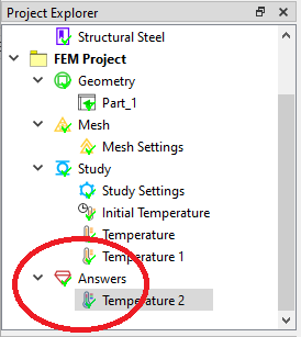
At the same time, the status of the solution object in the project window is updated, a green checkmark indicates that the solving succeeded.
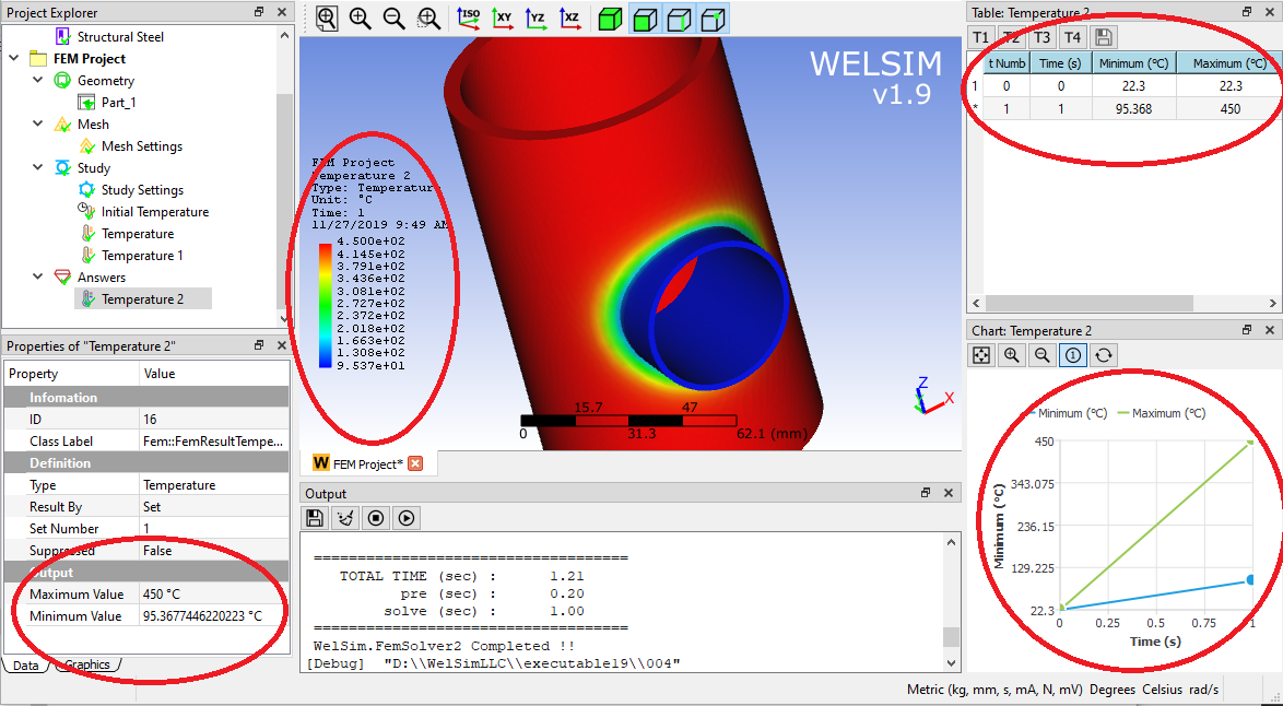
You can quickly review the temperature distribution by adding a result object. In the steady-state thermal analysis, you can get the temperature distribution, and the maximum and minimum temperature. As shown in the figure below, the temperature distribution and the maximum and minimum temperatures are displayed in different areas for easy reviewing.
In this article and example, we see that with the help of finite element analysis tools, nonlinear heat transfer analysis is not as difficult as it looks. The example defines the nonlinear thermal conductivity, solves the model, and reveals the temperature distribution on the structures.