When a finite element analysis model contains hyperelastic materials, engineers usually have little substantial data to help get the results. Sometimes a lucky engineer will have some tension or compression stress-strain test data, or simple shear test data. Processing and applying these data is a critical step to analyze the hyperelastic models. Particularly, the curve-fitting of these data to obtain the material constants is of importance. In this article, we will learn about the test data related to the hyperelastic model and its curve fitting. An example of curve-fitting in MatEditor will be given at the end of this article.
Mechanical test data of hyperelastic materials
The material constants in the strain-energy function determine the mechanical response of the selected hyperelastic model. To obtain correct analysis results, we need to evaluate material constants from the tested samples. These constants are usually obtained from the curve-fitting on the experimental strain-stress data. These test data are generally taken from several deformation modes over a wide range of strains. The material constants could be fit using test data in at least as many deformation states as will be experienced in the finite element analysis.
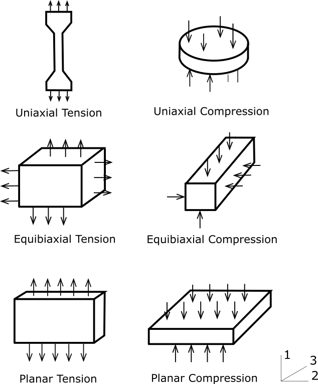
For hyperelastic materials, simple deformation tests can be used to characterize the material constants. The six different deformation modes are graphically illustrated in the figure below. The combination of multiple tests will enhance the characterization of the hyperelastic behavior of a material.
Although there are six different deformation modes, we found that after applying hydrostatic pressure, the following modes become identical: uniaxial tension and equibiaxial compression, uniaxial compression and equibiaxial tension, planar tension and planar compression. With these equivalent test modes, we now have only three independent deformation modes for which one can get test data.
Uniaxial tension (Equibiaxial compression)
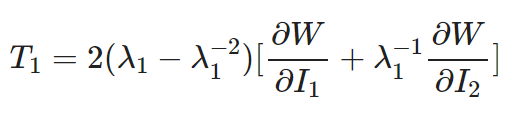
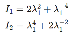
This is a type of simple tensile test stress-strain data with no lateral constraints. Such test data must be provided to calculate the tension deformation. Uniaxial compression data can be derived from equibiaxial data.
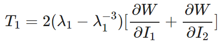
For uniaxial tension, The first and second strain invariants become:
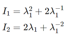
The corresponding engineering stress can be expressed using the principal stretch ratio:
Equibiaxial tension
Stress-strain data in a biaxial tension test. By stretching uniformly in two directions, the strain state is equivalent to pure compression. Equibiaxial compression data can be derived from uniaxial tension data.
For equibiaxial tension, The first and second strain invariants become:
The relationship between the corresponding engineering stress and the principal stretch rate is:
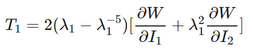
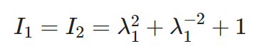
Pure shear deformation
For hyperelastic materials, shear deformation refers to a sample that is heavily stretched, but since the material is almost incompressible, there is a pure shear state.
The first and second strain invariants are:
The relationship between the corresponding engineering stress and the principal stretch rate is:
Volumetric deformation
This data is used to determine the bulk modulus. For hyperelastic materials, this data is more important if the material can be slightly compressed or the whole geometry model is constrained. The bulk modulus is usually 2–3 orders greater than the shear modulus. For foam materials, volumetric data becomes important for calculating the compressibility of the material.
Hyperelastic model and curve fitting
The number of material constants and physical meanings are different between hyperelastic models, we list the strain energy of each hyperelastic model for clarification purposes. Currently, MatEditor has already supported the following hyperelastic models.
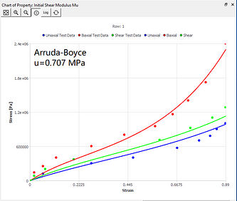
Arruda-Boyce model
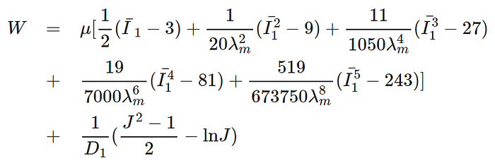
where u is the initial shear modulus, lambda is the limiting network stretch, and D1 is the material incompressibility parameter.
Blatz-Ko model
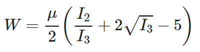
where u is the initial shear modulus of the material.
Gent model
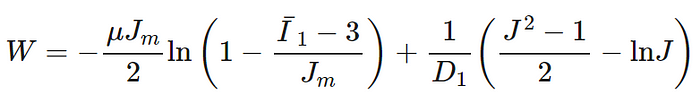
where u is the initial shear modulus, Jm is the limit value of I1–3, and D1 is the material incompressibility parameter.
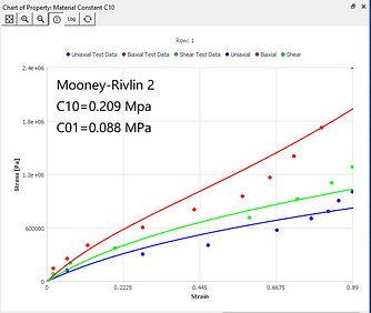
Mooney-Rivlin 2-parameter model
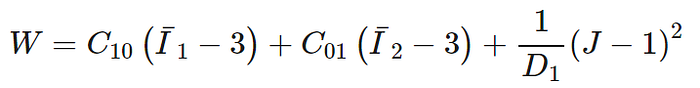
where C10, C01, and D1 are material constants.
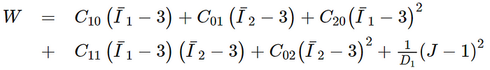
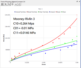
Mooney-Rivlin 3-parameter model

where C10, C01, C11, and D1 are material constants.
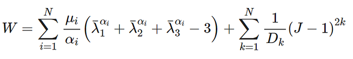
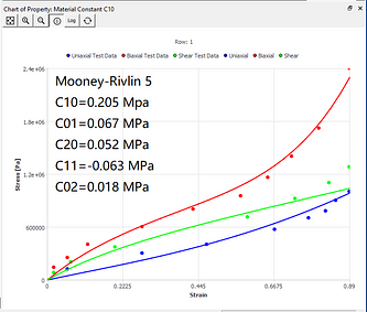
Mooney-Rivlin 5-parameter model
where C10, C01, C20, C11, C02, and D1 are material constants.
Mooney-Rivlin 9-parameter model
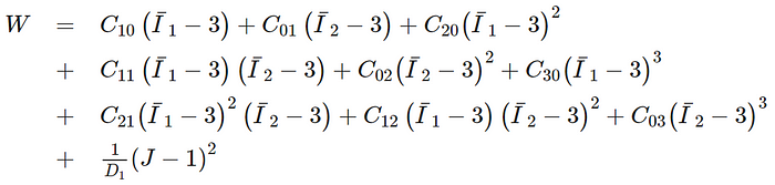
where C10, C01, C20, C11, C02, C30, C21, C12, C03, and D1 are material parameters.
Neo-Hookean model
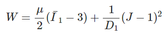
where u is the initial shear modulus of materials, D1 is the material incompressibility constant.
Ogden model
where N determines the polynomial order, u_i and a_i are material constants, and Dk is the incompressibility parameter.
Polynomial model
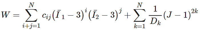
where N determines the order of the polynomial, and c_ij and D_k are material constants.
Yeoh model
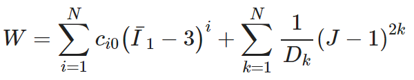
where N denotes the order of the polynomial, and c_i0 and D are material constants.
Based on specific conditions, you can accurately calculate material constants by combining the measured data of uniaxial tension, biaxial tension, pure shear, and volumetric deformation. These test data can then be curve-fitted for each hyperelastic model.
Given the test data and the specific hyperelastic model, the material constants can be calculated by the least square analysis to obtain the optimized results. The Levenberg-Marquardt solver is commonly used to minimize the residual of the curve fitting. This curve-fitting scheme is one of the most effective methods in finding hyperelastic material constants; however, the stability should also be considered. The Drucker stability criterion is widely applied to determine the stability of the hyperelastic material model. According to the Drucker criterion, the strain energy associated with the incremental stress should be greater than zero. The material model can be unstable if this criterion is not satisfied. In the numerical practices, checking for the stability of a material can be more conveniently accomplished by checking for the positive definiteness of the material stiffness.
Use MatEditor to fit hyperelastic material curves
The engineering material editing software MatEditor has supported a variety of hyperelastic models and curve fitting. By inputting the stress-strain test data, the hyperelastic material constants for finite element analysis can be obtained. MatEditor cannot only solve the curve-fitting for the test data but also plot the fitted curves and the test data in the same chart window, which is convenient for comparison and examination. In this way, the user can quickly obtain the hyperelastic material constants from the experimental stress-strain data.
Currently, the hyperelastic curve fitting models supported by MatEditor and WelSim are Arruda-Boyce, Mooney-Rivlin, Neo-Hookean, Ogden, Polynomial, and Yeoh models. This example uses the Mooney-Rivlin 9 as an example. The fundamental steps of curve fitting are as follows:
1) Choose a hyperelastic model
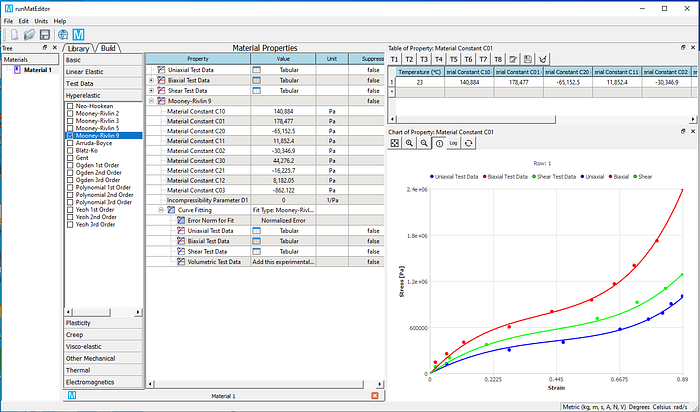
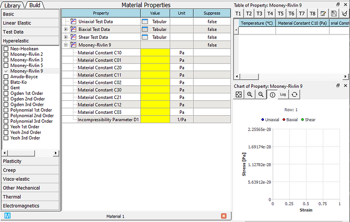
Select the Mooney-Rivlin 9 material property from the hyperelastic toolbox and add it to the material properties editing window. The material constants at this time are blank and require the user’s input or parameter fitting.
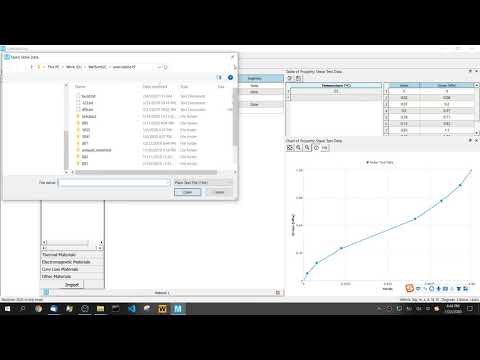
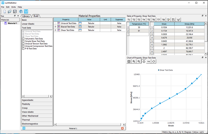
2) From the test data toolbox, choose to add three types of test data: Uniaxial, Biaxial, and Shear Test Data, and enter the test values in the table, as shown in the figure below for shear test data. MatEditor also supports test data at multiple temperatures. These test data needs to cover the entire strain range of subsequent simulations. For the massive test data, the user also can import strain-stress data by loading a file.
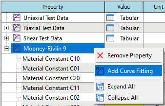
3) After confirming that the test data is entered correctly. Right-click Mooney-Rivlin 9 property and add a Curve Fitting property.
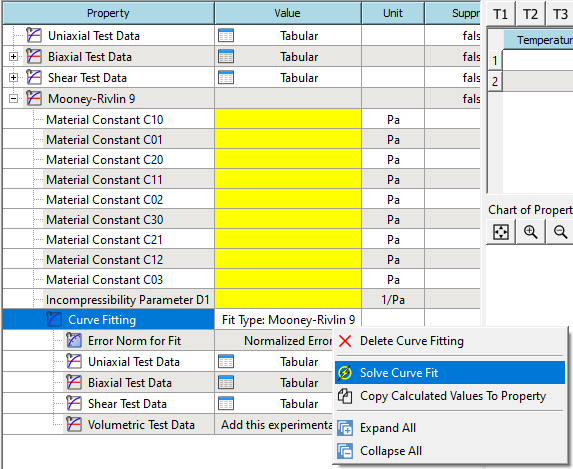
4)Right-click the Curve Fitting property that you just added, Solve, and Copy the Calculated Value to the material property.
5) If the solving and assignment are successful, you can view the material parameters and curves after fitting.
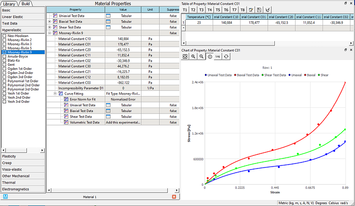
6) Compare the difference between the solved curves and the test data. And decide whether to use these constants for subsequent analysis. In this example, nine parameters of Mooney-Rivlin have been calculated. The volumetric deformation data is used to calculate the incompressibility parameter D, which can be obtained by curve fitting of volumetric test data. If there is no volumetric test available, then D=0. In this case, you may need to manually modify the value of D. If you know the Poisson’s ratio v, you can use the following formula to calculate: d=(1–2v)/(c1+c2). Note that this formula is based on the assumption of incompressibility (v is close to or equal to 0.5).
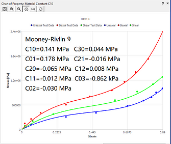
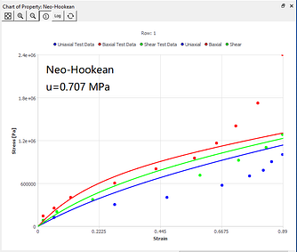
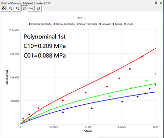
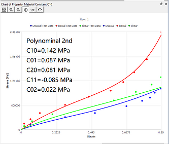
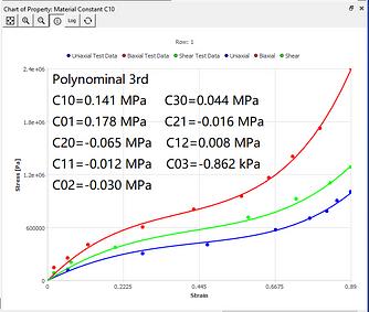
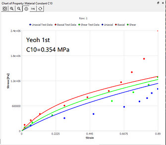
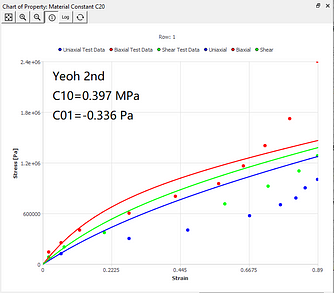
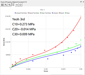
The curve fitting results of different models under the same set of data sources are now given. You can intuitively understand the characteristics of curve fitting of different hyperelastic models.
| — | —- | — |
|  |
|  |
|  |
|
|
|  |
|  |
|  |
|
|
|  |
|  |
|  |
|
|
|  |
|  |
|  |
| — | —- | — |
|
| — | —- | — |
Notes on curve fitting of the hyperelastic model
1) To obtain accurate material constants, the stress-strain data entered in the curve fitting must cover the complete load range that will be encountered in the analysis. For example, if the finite element analysis model is subjected to the shear stress in addition to tension and compression, you may need to enter pure shear data for curve fitting. Simple tension data alone is not sufficient to model material behavior in complicated deformation modes. If you only fit uniaxial data and use the calculated parameters for the biaxial deformation analysis, you may get incorrect simulation results. In material constant estimation, it is better to perform curve fitting in combination with different large deformation modes, rather than using only one deformation mode.
2) In most cases, the curve fitting routine cannot achieve perfect accuracy. The result of curve fitting depends largely on the test data given in the required range.
3) Most of the hyperelastic models are based on the incompressibility assumption (except for Blatz-Ko and Ogden Foam models, etc.). For these models, when inputting parameters, pay attention to the Poisson’s ratio should be close to 0.5, generally greater than 0.49. In this way, reasonable results can be obtained in finite element analysis.
In this article, we discussed various hyperelastic models and curve fittings for hyperelastic materials. To fit the material constants to the material model, we need correct measurement data. We also analyzed some typical experimental tests and hyperelastic material models. Through examples in the MatEditor software, it is demonstrated how to directly use the test data in the nonlinear hyperelastic model and fit the parameters of different hyperelastic models.
In the end, a video tutorial about using MatEditor curve fitting is given for your reference.