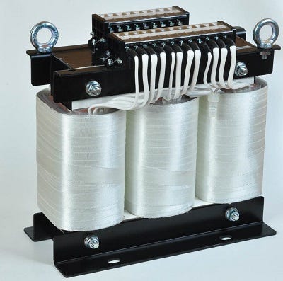
The core loss of magnetic components plays an important role in engineering practices. Particularly at high-frequency conditions, the loss of magnetic components accounts for a large proportion of the energy loss of the whole unit. Most manufacturers provide the core loss curve in the product manuals. The core loss also has corresponding theoretical models and coefficients. Some core material manufacturers give these coefficients, but some manufacturers do not provide it. In this scenario, the user needs to perform curve-fitting on the core loss curves to obtain the parameters by themselves. The core loss is also a common factor in electromagnetic simulation, especially in the post-processing analysis of the electromagnetic results, the fitted coefficients of core loss are commonly used.
Core loss is closely related to magnetic material characteristics and operating frequency. Equally, the core loss is also related to working temperature. There are valid methods for calculating core loss at different temperatures. This article focuses on the curve fitting of the core loss P-B test data. The effect of temperature on energy loss will be described in a future article.
Models and numerical methods of core loss curve fitting
Common core loss models include the classical model, Steinmetz model, and modified Steinmetz models, etc. Since these models are similar, this article will only focus on the theoretical and numerical methods of the classical and Steinmetz models.
Computation of electrical steel core loss from loss curves
The iron-core loss without DC flux bias is expressed as the following:

where Bm is the amplitude of the AC flux component, f is the frequency, Kh is the hysteresis core loss coefficient, Kc is the eddy-current core loss coefficient, and Ke is the excess core loss coefficient. Hysteresis loss (Ph) is the energy loss caused by the magnetic domain during the magnetization process of the magnetic domain to overcome the friction between the magnetic domains. This part of the loss eventually heats the component and dissipated. The energy lost per unit volume of the core is proportional to the area enclosed by the hysteresis loop. Each magnetization cycle consumes energy proportional to the area enclosed by the hysteresis loop, so the smaller the hysteresis curve area is, the smaller the hysteresis loss is; the higher the frequency, the greater the power loss. Eddy current loss (Pc) is due to the resistivity of the magnetic core material is finite, and has a certain resistance. At high frequencies, the eddy current in the magnetic core will be caused by the exciting magnetic field and lead to losses. Residual loss (Pe) is a loss due to the magnetization relaxation effect or magnetic hysteresis effect. The so-called relaxation means that during the process of magnetization or demagnetization, the magnetization state does not immediately change to its final state with the change of the magnetization intensity, but requires a process. This ‘time effect’ is the cause of excess loss.
For the given P-B test data, as long as the quadratic form below is minimized, the curve parameters Kf, Kc, and Ke can be obtained.

where m is the number of loss curves, n_i is the number of data points for the i-th loss curve, and p_ij is a two-dimensional look-up table for loss curves.
Computation of power ferrite core loss (Steinmetz model)
Although the classical method gives a reasonable explanation of magnetic core loss, it is inconvenient to calculate certain magnets in the practices. The mathematician and electrical engineer Steinmetz summed up an empirical formula suitable for engineering calculation of core loss. The expression is as follows:
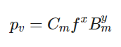
where p_v is the average power loss density, f is the excitation frequency, and Bm is the peak magnetic flux density. This formula shows that the loss per unit volume p_v is an exponential function of the repetitive magnetization frequency and magnetic flux density. Cm, x, and y are empirical parameters. Both exponents can be non-integer, generally 1<x<3 and 2<y<3. For different materials, manufacturers generally give a corresponding set of parameters. This formula is commonly used to represent the state of magnetization under sinusoidal excitation and cannot be used for non-sinusoidal magnetic excitations such as square waves. The Steinmetz model has only three parameters and has proved to be a useful tool for calculating core loss. For the sinusoidal waveform, it is more convenient and accurate to calculate the core loss using this formula.
To linearize the equation for curve fitting, we used base-10 logarithms. The equation above can be rewritten to
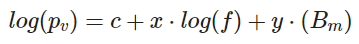
where c=log(Cm)。
By minimizing its quadratic form below, its parameters c, x, and y can be calculated.

where m is the number of loss curves, n_i is the number of points of the i-th loss curve, and p_vij is a two-dimensional look-up table for loss curves. Then coefficient Cm is calculated from the equation c=log(Cm).
The numerical algorithms for function minimization involve more content, which we will discuss in future articles.
Procedures of core loss curve fitting
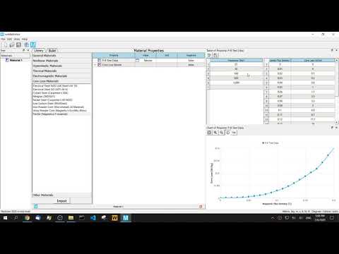
The following describes how to use MatEditor to fit the parameters of the core loss curves. MatEditor is a free engineering material data editing software. The same module is also included in the finite element analysis software WelSim.
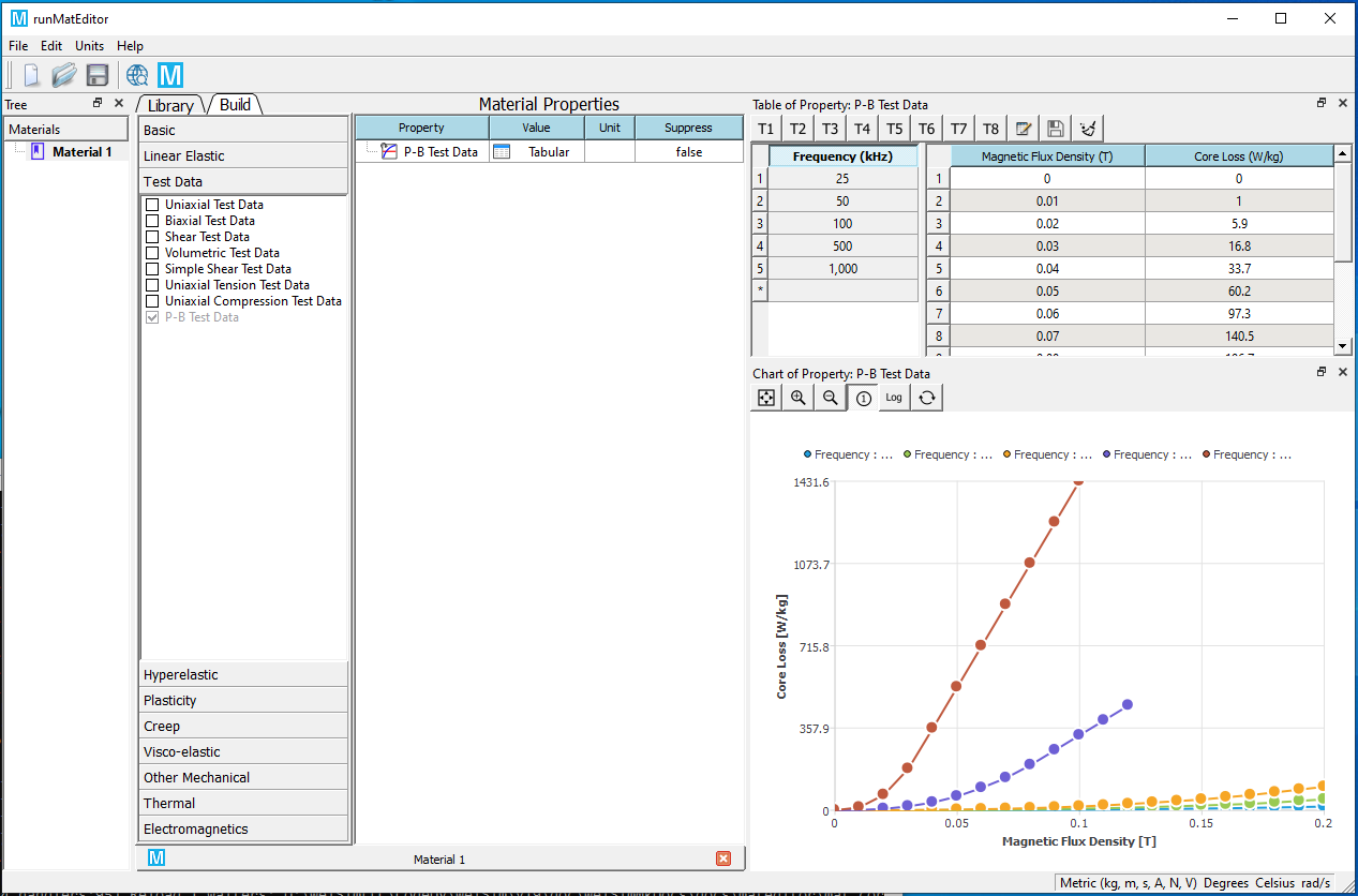
Add P-B Test Data material property, and input the data into the table, these data are often from the manufacturer’s manual of magnetic products. You can also enter table data by loading a text or Excel file. After inputting, click the frequency of each line, and the chart window will display the related P-B curves. Clicking on the header of the frequency column will display all P-B curves together.
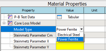
2) Add Core Loss Model material property and set Electrical Steel or Power Ferrite in the Model Type.
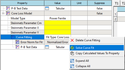
3) Right-click the Core Loss Model property pop-up menu and add Curve Fitting sub-property.
4) After adding the curve fitting sub-property, right-click, and select Solve Curve Fit from the pop-up context menu to solve the curve fitting.
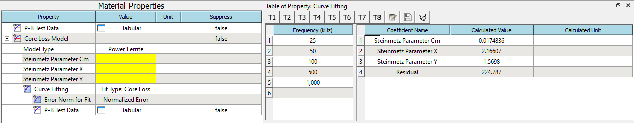
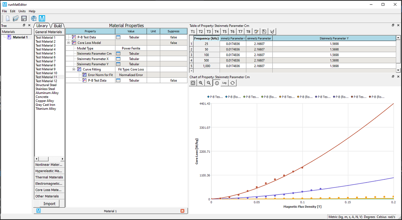
5) If the solving succeeds, the calculated coefficients will be automatically displayed in the table window. As the picture shows,
6) Right-click on the curve fitting property and select Copy Calculated Values to Property. The calculated coefficients will be set to the coefficient properties.
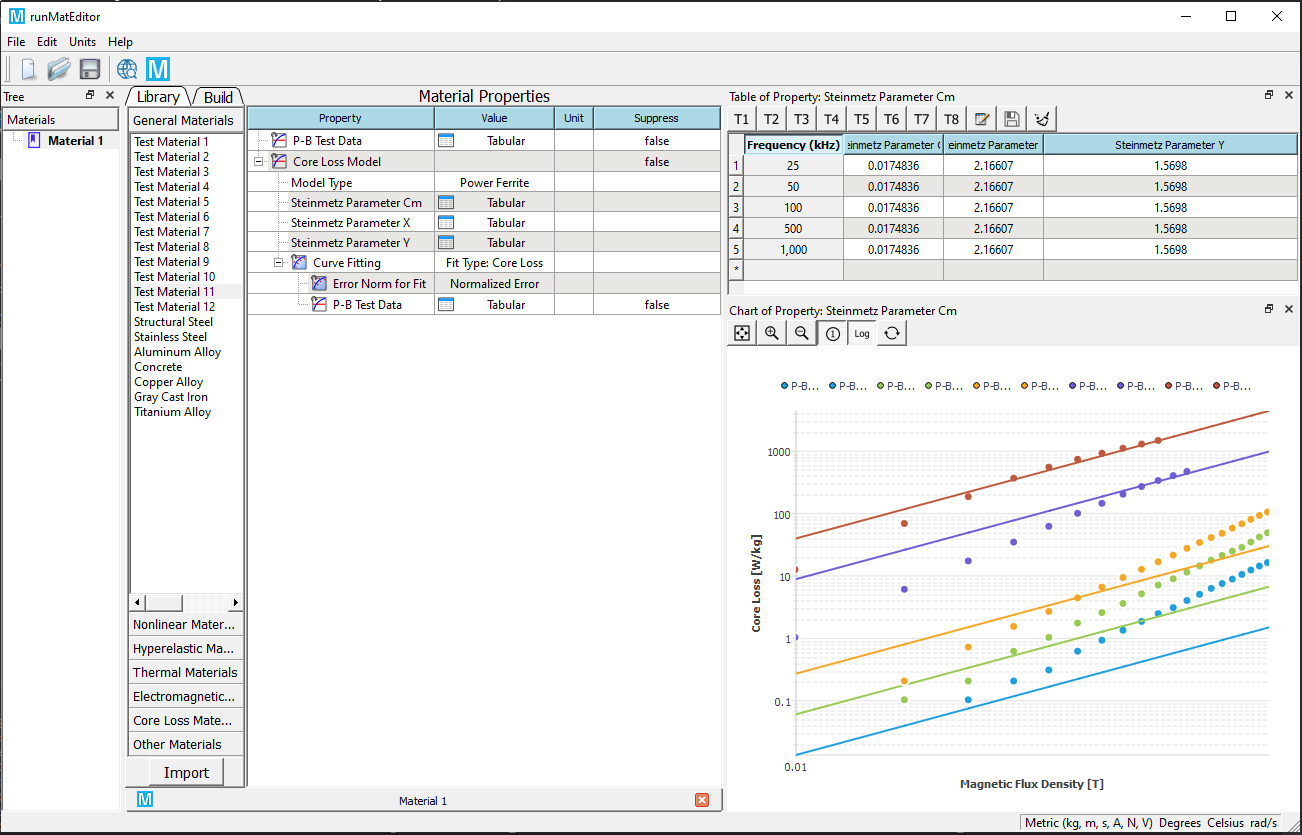
7) (Optional) For the magnetic core material, we often need to display the curves in the logarithmic axis. Click the logarithmic axis button to display the curves in the logarithmic axis.
This case uses the Power Ferrite (Steinmetz) model as an example. The curve fitting procedures for the Electrical Steel model are the same.
A tutorial video is attached below for your reference.