Curve fitting is a numerical process often used in data analysis. Its essence is to apply a certain model (or called a function or a set of functions) to fit a series of discrete data into a smooth curve or surface, and numerically solve the corresponding parameters, thereby obtaining the relationship between the coordinates represented by the discrete points and the function. Curve fitting can help us understand the internal connection between data and predict the trend of such problems. In the practice of data analysis, most of the curves or surfaces that need to be fitted are nonlinear, so computer programs are required to obtain results.
The curve fitting has been widely applied in many areas, particularly in nearly every sector of statistical analysis. For examples, various lines and curves fitting in image processing, vibration and noise data processing in mechanical engineering, prediction of financial and sales data, the quantity of drug inhibitor on the induced cell change, the concentration of medicine and time, the efficacy of medical treatment and treatment duration, competition between species, etc. Curve fitting can apply to help us better understand many of these problems. In addition, in the field of structural finite element analysis, various nonlinear material parameters are obtained by parameter fitting from test data. In the electromagnetic analysis, the core loss parameters are curve fitted from the test data between power loss and magnetic flux density.
Common Curves (Functions)
Here is an introduction to the types of curves that are often encountered in data analysis, including linear and nonlinear. Of course, we know that most models in curve fitting are nonlinear. The CurveFitter from WelSim already supports the fitting calculation of these curves.
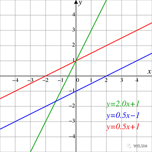
1) Straight line
The straight-line y=A+B*x is one of the simplest regression models in curve fitting, where x is the independent variable, y is the dependent variable, and A and B are the parameters to be fitted. Its main goal is to find the general direction of data concentration and data growth.
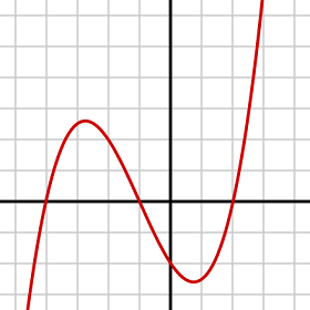
2) Polynomial
The polynomial y=A+B1x+B2x2+……+Bk*xk is a commonly used model in various engineering areas, where x is the independent variable, y is the dependent variable, the order number k is often between 1–9. When the order is 1, the polynomial becomes a straight line. When the order is greater than 1, the model exhibits nonlinearity. The higher the order, the more complex the curve can be represented. However, higher-order polynomials require more test data points to get accurate solutions, and it also results in expensive computation. In practice, an appropriate order should be chosen according to the data source and target problem.
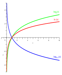
3)Logarithm
Generally, the logarithmic model has two different forms: semi-logarithmic y=Alg(x)+B and full logarithmic lg(y)=Alg(x)+B, where x is the independent variable, y is the dependent variable, and A and B are the parameters to be fitted. The logarithmic curve is often used in models related to changes in concentration.
4)Power
There are two common power functions: y=Ax^B and y=Ax^B+C, where x is the independent variable, y is the dependent variable, and A, B, and C are the parameters to be fitted. The power function is widely applied in many fields. Scholars have found that the resting metabolic rate of an animal has a power function relationship with its body weight, and the size of the tumor and the rate of change also have a power function relationship.
5) Exponential
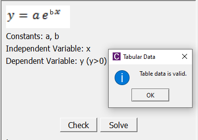
Common exponential functions are: y=Ae^(Bx) and y=Ae^(Bx)+Ce^(D*x), where x is the independent variable, y is the dependent variable, and A, B, C, and D are the parameters to be fitted. The exponential can be used to express the relation between nutrition and human health.
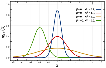
6) Normal distribution
One of the most common normal distribution is Gaussian model y=A*e^[-(x-B)²/C²], where x is the independent variable, y is the dependent variable, and A, B, and C are the parameters to be fitted. A large number of normal distribution models are used in statistics, such as the relationship between children’s height and body density, the distribution of students’ test grades, and so on.
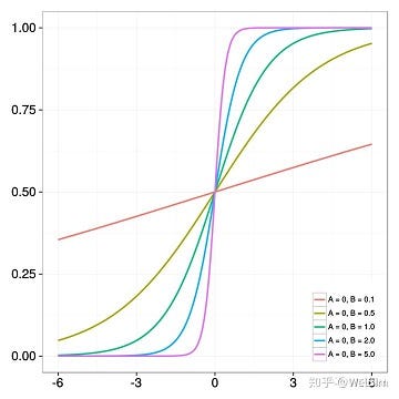
7) Sigmoid
The commonly used sigmoidal curves are symmetrical and asymmetrical types, which are also called 4-parameter and 5-parameter logistic regression functions. The mathematical expressions are y=D+(AD)/[1+(x/C)^B] and y=D+(AD)/[1+(x/C)^B]^M respectively, x is the independent variable, y is the dependent variable, and A, B, C, D, and M are the parameters to be fitted. Depending on the values of parameters, the shape of the curve may be a monotonously increasing exponential, logarithmic, or hyperbolic curve, it may be a monotonously declining curve or a sigmoidal curve. It requires that the value of x cannot be less than 0 (because the exponent is a real number). Because of its versatility, sigmoid has also become one of the commonly used curves in scientific research or engineering.
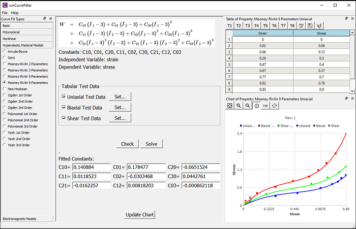
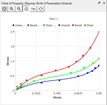
8) Hyperelastic material models
The popular hyperelastic models include Arruda-Boyce, Gent, Mooney-Rivlin, Neo-Hookean, Ogden, Polynomial, and Yeoh, etc. The independent and dependent variables are strain and stress, respectively. According to different hyperelastic models, the curves could be entirely different. In the finite element analysis, due to the diversity of hyperelastic materials, it is difficult to directly have the material parameters from the manual or literature, but the mechanical test data of those hyperelastic materials can be obtained from experiments. Fitting these test data can give us material constants for the successive finite element analysis. Since the mechanical test data has multiple deformation types, it is necessary to calculate and fit the stress-strain curve at various deformation types. Interested readers can get more information from CurveFitter’s user manual.
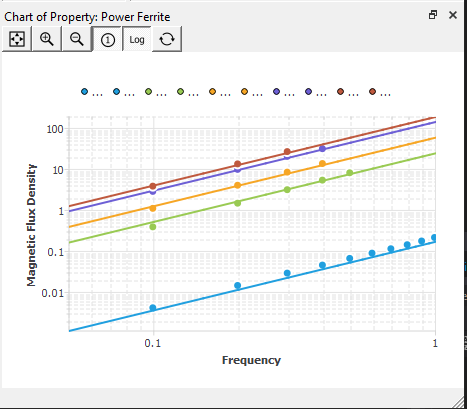
9) Core loss model curve
The loss of magnetic core material has some classic models such as p=KffBm²+Kc(fBm)²+Ke(fBm)^{1.5} for electrical steel, and power ferrite p=Cmf^XBm^Y, where Bm is the independent variable, p is the dependent variable, f is the input electromagnetic frequency, Kf, Kc, Ke and Cm, X, Y are the parameters to be fitted. The latter is also known as the Steinmetz model. Similar to the hyperelastic curve fitting, the core loss curves may need to fit multiple sets of test data at a time.
Curve Fitting Tool — CurveFitter
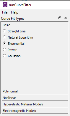
Although curve fitting is widely used in many fields, there is no easy-to-use and free curve fitting software. The finite element software WelSim has just released a free curve fitting tool, CurveFitter, which is extracted from the curve fitting module for complex hyperelastic material and core loss models. CurveFitter has added many curve models and becomes an independent software application dedicated to generic curve fitting for a wider range of scientific and engineering applications.
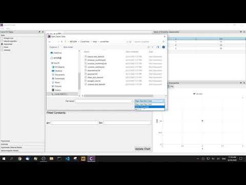
The steps to use CurveFitter are as follows:
1) Select the curve equation to be fitted from the toolbox
2) Edit and input table data, or import data from files directly.
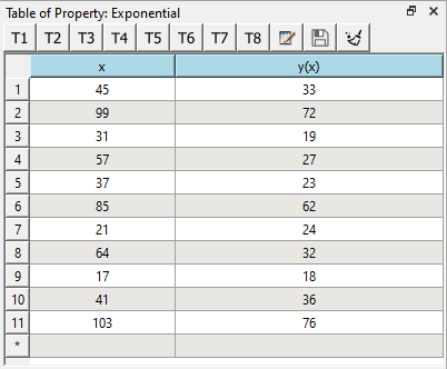
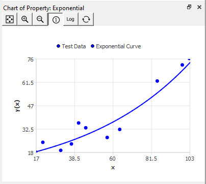
3) Check the input test data in the chart window.
4) Click the check button to check the test data (optional). A pop-up dialog box will prompt the status.
5) Click the Solve button to perform the numerical calculation of curve fitting. If the solution is successful, the parameter fields will automatically display the fitted values, and the chart window will display the fitted curve.
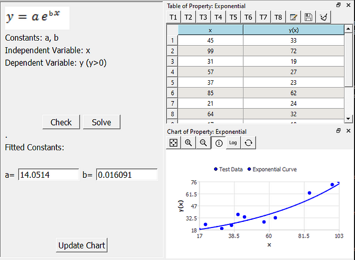
6) So far the curve fitting calculation has been completed. If you would check the shape of the curve with different parameters. You can adjust the value of the parameter field and click the update button.
Discussion
In curve fitting, it is best to choose a function model based on the shape of the curve. A different fitting function results in different precision and parameters. We need to choose the best fitting function according to the optimal principle. It is also important that the number of given data points and the range of data points also affect curve fitting. Due to the error of the fitted data, it is necessary to check the fitted curve and parameters after calculation. We also need to minimize the influence of model errors and measurement errors on curve fitting.
Finally, the operation video is attached for your reference.