Modern electromagnetic research has penetrated various fields. In recent years, with the rapid development of new technologies such as 5G, electric vehicles, and IoT, the role of electromagnetic analysis has become more and more important. Electromagnetics simulation has been widely and successfully applied to many aspects of electromagnetic performance prediction and design. Under the premise of reasonably setting the model and parameters, electromagnetic simulation can replace experiments in many aspects, and provide great help for the rapid development of electromagnetic devices.

Although electrostatics is a relatively simpler type of electromagnetic analysis, it has a wide range of applications and acts as the basis for other types of electromagnetic analysis. As an important part of electromagnetics, electrostatics is as abstract and difficult to be understood as the magnetic field. In particular, the electrostatic induction phenomenon of conductors in the electrostatic field also makes electrostatic analysis more complicated.
Using finite element simulation technology, you can quickly and accurately calculate the electrostatic field distribution under many specific occasions or conditions. For example, calculation of electronic components such as capacitance and inductance analysis, the design of various types of cables, electromagnetic shielding, electromagnetic compatibility, lightning protection device design, etc. have many applications. Especially with the increase in the capacity and working voltage of electrical equipment, electrostatic simulation becomes more necessary. Electrostatic simulation can predict performance indicators such as the insulation, discharge, and breakdown possibility of the equipment.
Numerical methods of three-dimensional electrostatic analysis
All electromagnetic field calculations are based on the well-known Maxwell’s equations, and the full form of this equation is too heavy for calculating the electrostatic field. After a series of simplifications and assumptions, the governing equation of the electrostatic field can be described as a Poisson equation to the electric potential:
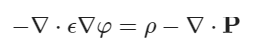
Where \phi is the electric potential, the unit under the international system of units is Volts, \epsilon is the permittivity, \rho is the charge source, and P is the polarization vector.

In the numerical methods of electromagnetics, the finite difference time domain (FDTD), method of moment (MoM), finite element method (FEM), and discontinuous Galerkin (DG) method are commonly used. Since the electrostatic problem is elliptic, according to the governing equation, the FEM is one of the best ways to solve it. At present, there is some general and specific finite element software on the market that can solve electrostatic problems. WELSIM has also supported the calculation of 3D linear electrostatic fields.
The material parameter commonly used in electrostatic field analysis is permittivity. The permittivity in a vacuum is 8.854e-12 F/m. Practical engineering also often uses relative permittivity to represent the dielectric properties of materials.
Commonly used boundary conditions and source excitation are:
1) Voltage
The voltage, the potential quantity in the governing equation, is a common piecewise boundary condition in electromagnetic analysis. It is a Dirichlet boundary condition.
2) Normal component of electric displacement
This normal component is equivalent to the surface charge density on the surface. This is rarely used because surface charge densities are rarely known unless they are known to be zero. However, if the surface charge density is zero then the Neumann BCs are not needed because this is the natural boundary condition.
3) Charge or charge density
An electric field source that provides potential excitation for the field, which can be positive or negative. Generally, it is a point or spherical charge.
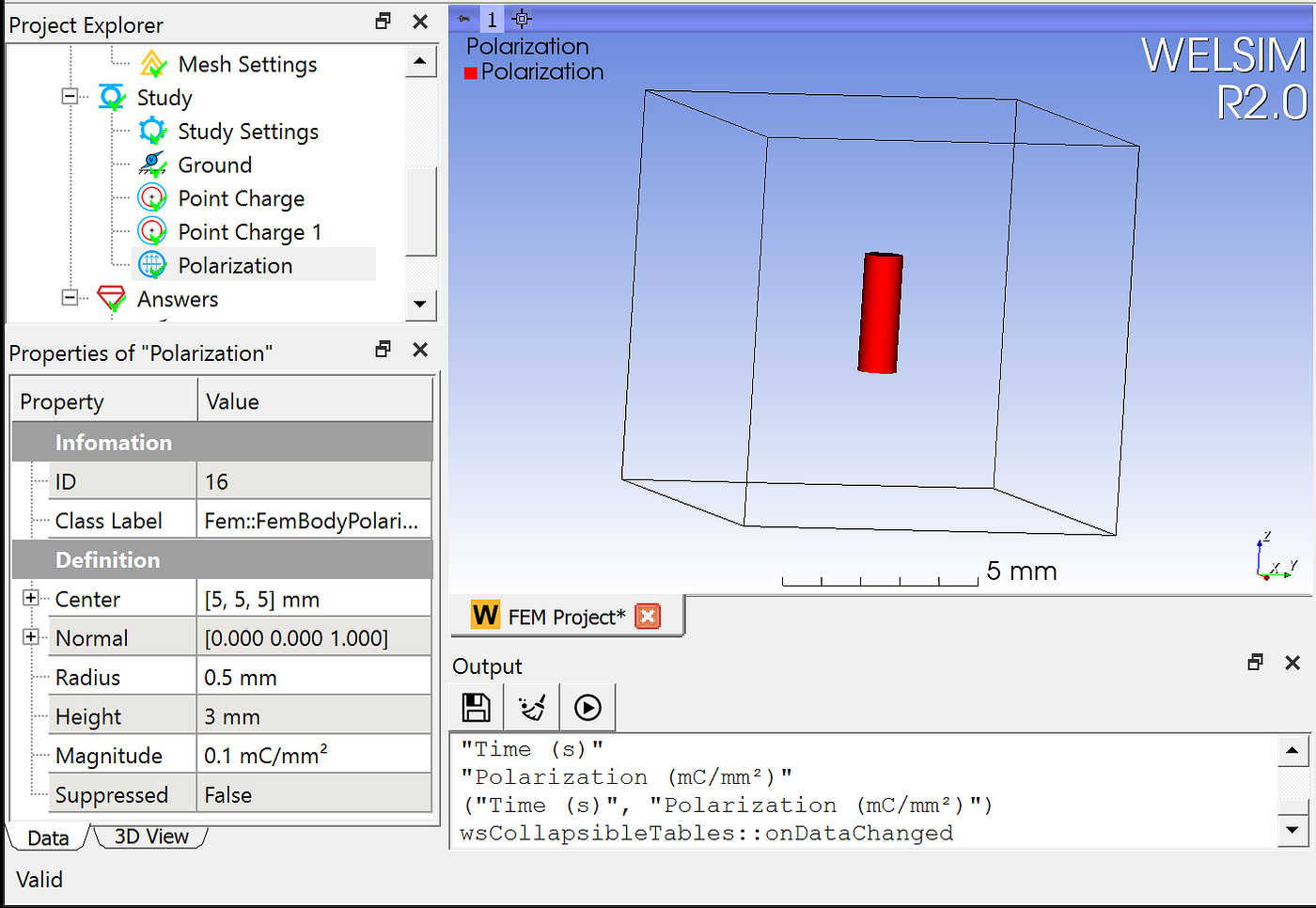
4) polarization
A polarization vector function can be imposed as a source of the electric field. Polarization can be created by a simple voltaic pile. Generally, a given position and size as well as the magnitude of the polarization are required to define this source.
Perform 3D electrostatic analysis using WELSIM
The electrostatic field analysis in WELSIM is very simple and convenient, and the electric field distribution results can be quickly obtained with a few simple operations.
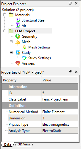
1) Create an electrostatic FEM project
Create a new FEM project and set the Physical Type to Electromagnetics in the properties of the FEM project, and the Analysis Type is set to the default Electrostatics.
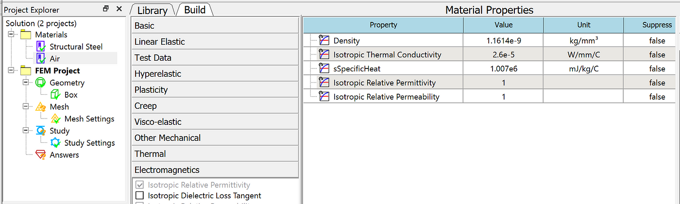
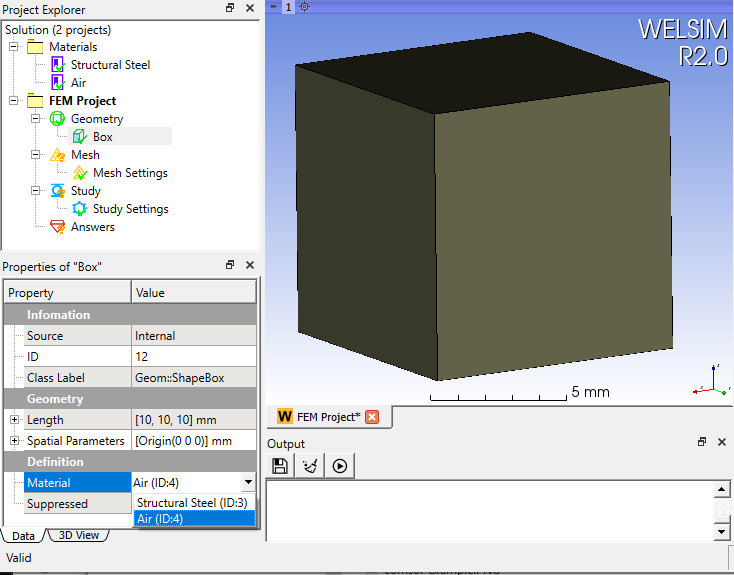
2) Define materials
In the electrostatic field analysis, the main material parameter is permittivity. Here we can open the default air material setting that comes with the system, where the relative dielectric constant has been set to 1, and you can use it directly.
3) Build a model
Create a 10x10x10 cm3 cube to simulate the electric field distribution. And set the cube material to air.
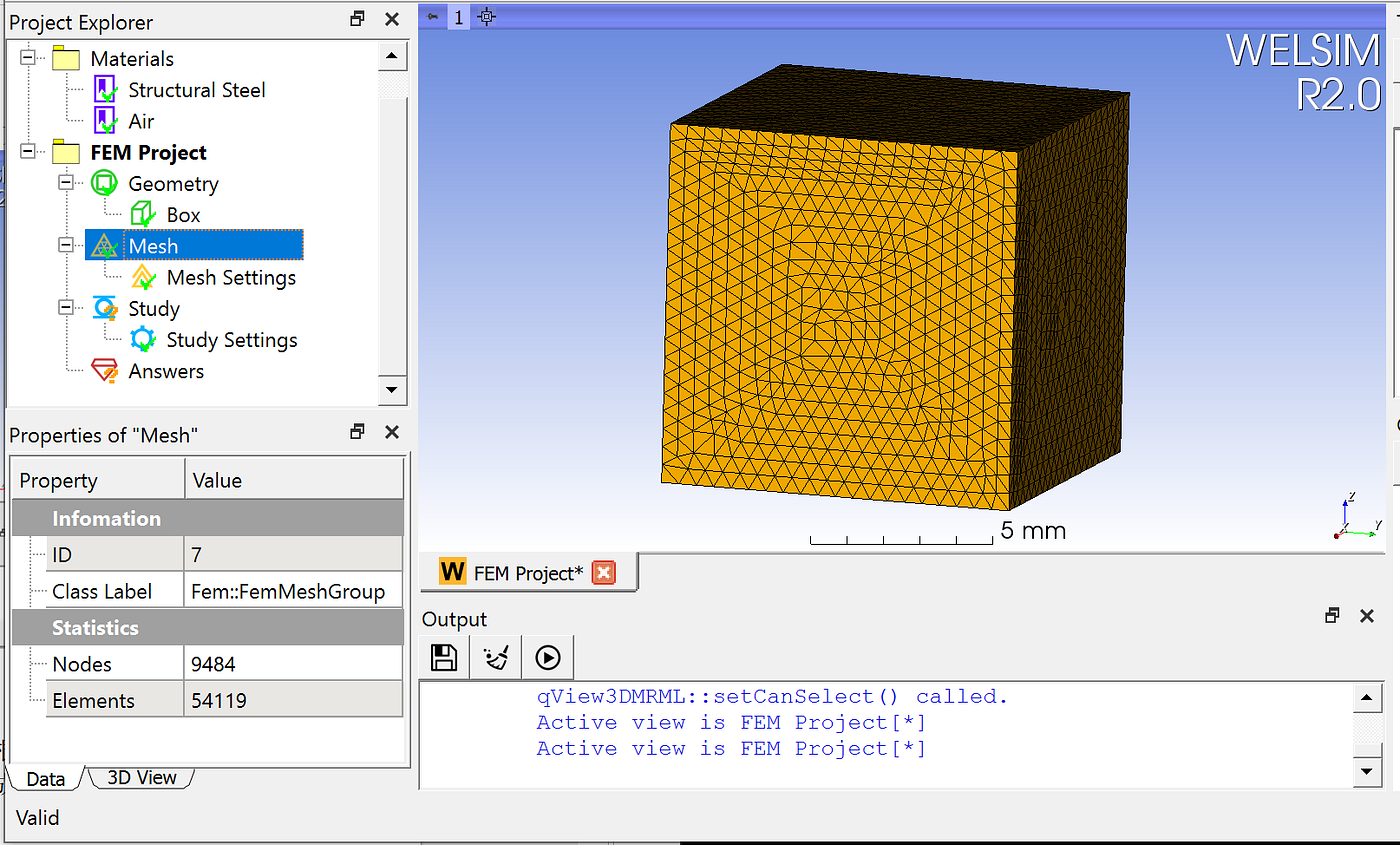
4) Mesh the domain
Set the maximum element size to 0.5 cm, and click the Mesh button. Since WelSim’s electromagnetic field solver will automatically use higher-order units according to the analysis type, there is no need to set higher-order elements here. After the meshing is completed, a total of 9484 nodes and 54119 Tet4 elements are generated.
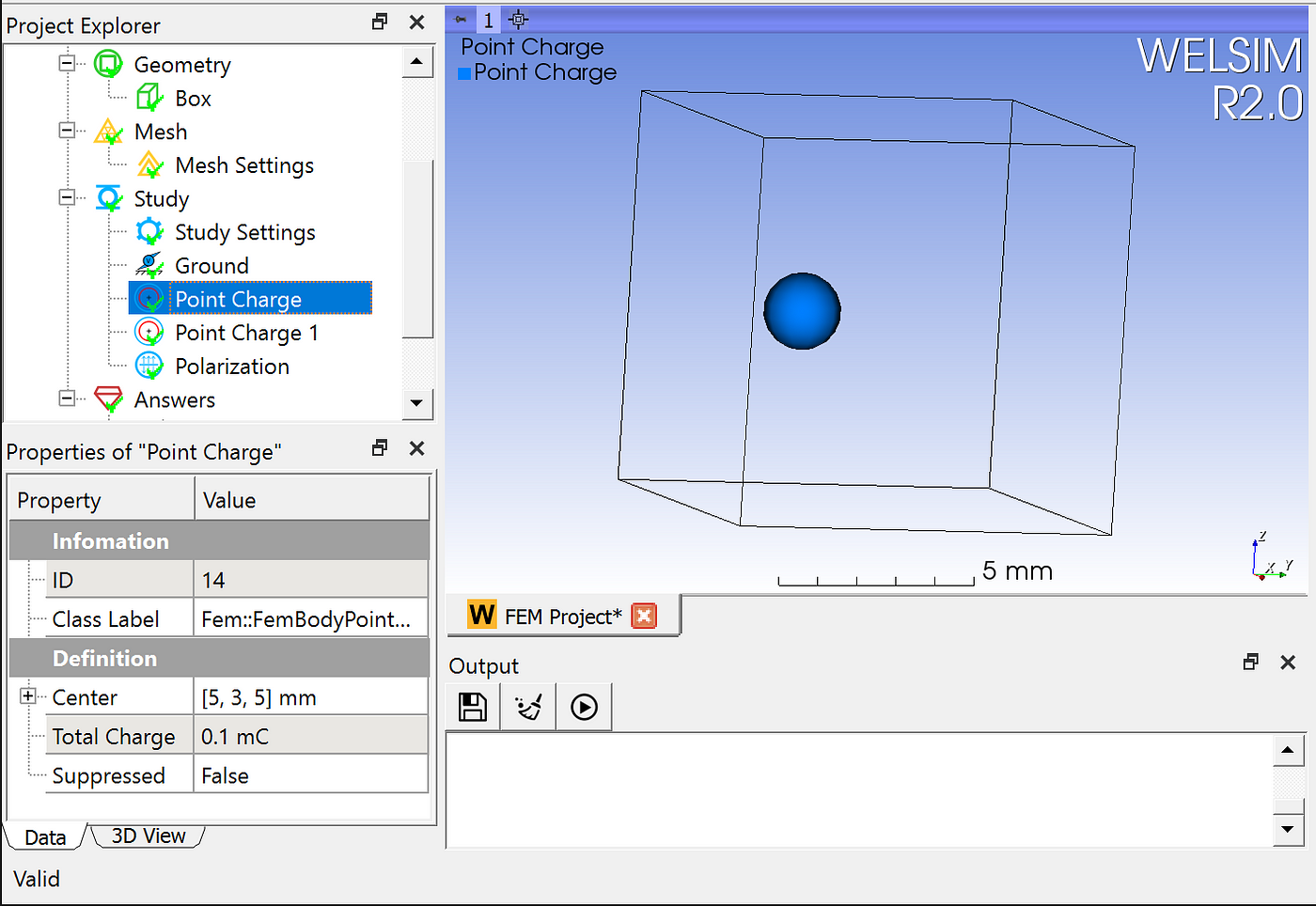
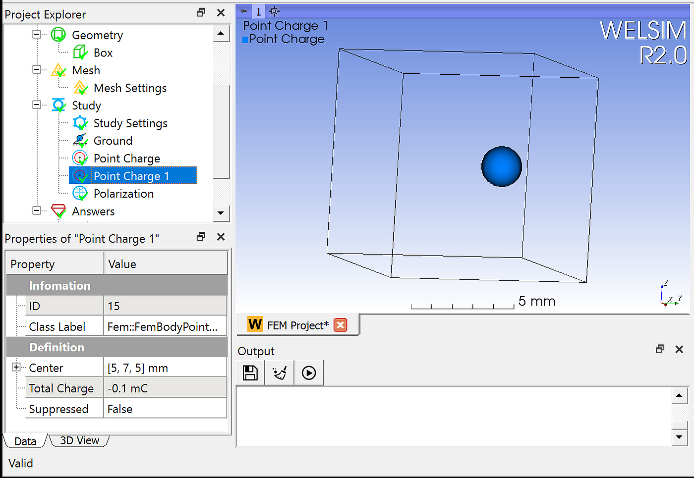
5) Impose boundary conditions or sources
The current version of WelSim supports voltage, zero potential (ground), and surface charge density boundary conditions, as well as a point charge, spherical charge, and polarization sources for electrostatic analysis.
Here we set
1) The peripheral zero voltage simulates the field at infinity.
2) Add two point charges and a cylindrical polarization inside the field.
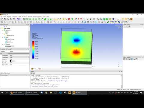
The point charges are 0.1 mC and -0.1 mC, respectively, and the magnitude of polarization is 0.1mC/mm2. The positions of the point charges and polarization cylinder are shown in the figures below.
6) Solve
Click the Solve button to perform the computation.
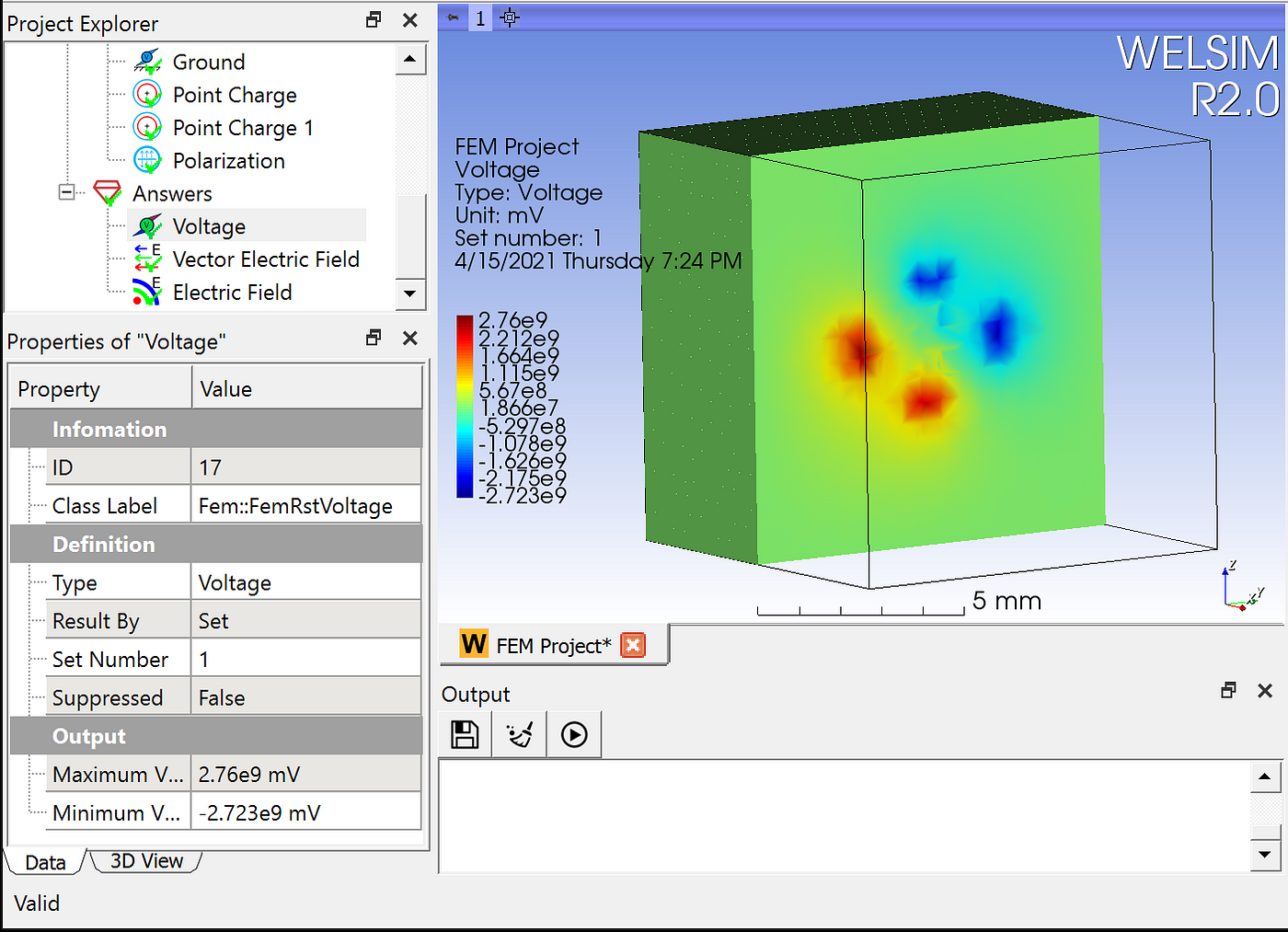
7) Evaluate the calculation results.
Add a voltage result to quickly evaluate the potential values. With post-processing tools such as clip planes, you can visually inspect the internal potential distribution inside the field. The maximum and minimum voltage values obtained here are 2.76e9 and -2.723e9 mV, respectively. The distribution of the potential is also consistent with the point charges and polarization conditions.
In addition to voltage results, the post-processing module of WelSim also supports electric field and electric displacement.
Finally, a video of the operation steps is given for reference.